The Art of Term Structure Models: Drift

After completing this reading, you should be able to:

• Construct and describe the effectiveness of a short-term interest rate tree assuming normally distributed rates, both with and without drift.
• Calculate the short-term rate change and standard deviation of the rate change using a model with normally distributed rates and no drift.
• Describe methods for addressing the possibility of negative short-term rates in term structure models.
• Construct a short-term rate tree under the Ho-Lee Model with a time-dependent drift.
• Describe the uses and benefits of the arbitrage-free models and assess the issue of fitting models to market prices.
• Describe the process of constructing a simple and recombining tree for a short-term rate under the Vasicek Model with mean reversion.
• Calculate the Vasicek Model rate change, the standard deviation of the rate change, the expected rate in T years, and half-life.
• Describe the effectiveness of the Vasicek Model.

In this topic, we delve into different term structure models used to estimate short-term interest rates. Specifically, we discuss models that have no drift (Model 1), constant drift (Model 2), time-deterministic drift (Ho-Lee), and mean-reverting drift (Vasicek).

Short-term Interest Rate Tree Assuming Normally Distributed Rates, Both With and Without Drift

Normal Distribution Without Drift

The simplest model for predicting the evolution of short rates, which we call Model 1, is used in cases where there is no drift, and interest rates are normally distributed. Under this model, the continuously compounded, instantaneous rate \(\text r_{\text t}\) is assumed to evolve according to the following equation:

$$ \text{dr}=\sigma \text{dw} $$

where:

dr = Change in interest rates over a small time interval, dt.

dt = Small time interval (measured in years) (e.g., one month = 1/12, 2 months = 2/12, and so forth).

\(\sigma\) = Annual basis-point volatility of rate changes.

dw = Normally distributed random variable with mean 0 and standard deviation \(\sqrt{dt}\).

Example: Estimating the Change in Short-term Rate

Assume that the current value of the short-term rate is 5.26%, that volatility equals 115 basis points per year, and that the time interval under consideration is one month or 1/12 years. Mathematically, \(\text r_0\) = 5.26%; \(\sigma\) = 1.15%; and dt = 1/12. A month passes and the random variable dw, with its zero mean and standard deviation of \(\sqrt{\frac {1}{12}}\) or 0.2887, happens to take on a value of 0.25. Determine the short-term rate after one month.

Solution

The change in the short-term rate is given by:

$$ \begin{align*} \text{dr} & =\sigma \text{dw} \\ & =1.15\%×0.25=0.2875\% \\ \end{align*} $$

Since the short-term rate started at 5.26%, the short-term rate after a month is 5.55%.

New short-term rate = 5.26% + 0.2875% = 5.55%

Since the expected value of dw is zero, it follows that the expected change in the rate, or the drift, is zero. Since the standard deviation of dw is \(\sqrt{\text{dt}}\), the standard deviation of the change in the rate is \(\sigma \sqrt{\text{dt}}\). For convenience, the standard deviation of the rate of change is sometimes referred to as the standard deviation of the rate. In the numerical example, the standard deviation of the rate is 0.332% or 33.2 basis points (= 1.15 × 0.2887).

Implication

Thanks to the definition above, it is possible to build an interest rate tree using a binomial model. We use equal probabilities of up and down movements from period to period (50% up and 50% down) and a recombining tree.

Interest Rate Tree With No Drift (Model 1)

A tree over dates 0 to 2 takes the following form:

$$ \textbf{Interest Rate Tree with No Drift} $$

$$ \begin{array} \hline {} & {} & {} & {\scriptsize {1/2} } & { r }_{ 0 }+2\sigma \sqrt { dt } \\ {} & {} & { \text r }_{ 0 }+\sigma \sqrt { \text { dt} } & {\Huge \begin{matrix} \nearrow \\ \searrow \end{matrix} } & {} \\ { \text r }_{ 0 } & {\begin{matrix} \scriptsize {1/2} \\ \begin{matrix} \begin{matrix} \quad \quad \quad \Huge \nearrow \\ \end{matrix} \\ \quad \quad \quad \Huge \searrow \end{matrix} \\ \scriptsize {1/2} \end{matrix} } & {} & {\scriptsize \begin{matrix} \begin{matrix} {1/2} \\\scriptsize \begin{matrix} \\ \end{matrix} \end{matrix} \\ \begin{matrix} \\ \end{matrix} \\ {1/2} \end{matrix} } & {{ \text r }_{ 0 }} \\ {} & {} & { \text r }_{ 0 }-\sigma \sqrt { \text {dt} } & {\Huge \begin{matrix} \nearrow \\ \searrow \end{matrix} } & {} \\ {} & {} & {} & {\scriptsize {1/2}} & { \text r }_{ 0 }-2\sigma \sqrt { \text {dt} } \\ \end{array} $$

The numerical example above, for example, leads to the following interest rate tree:

$$ \textbf{Numerical Example of Interest Rate Tree With No Drift} $$

$$ \begin{array} \hline {} & {} & {} & {\scriptsize {1/2} } & { 5.924\% } \\ {} & {} & { 5.592\% } & {\Huge \begin{matrix} \nearrow \\ \searrow \end{matrix} } & {} \\ { 5.26\% } & {\begin{matrix} \scriptsize {1/2} \\ \begin{matrix} \begin{matrix} \quad \quad \quad \Huge \nearrow \\ \end{matrix} \\ \quad \quad \quad \Huge \searrow \end{matrix} \\ \scriptsize {1/2} \end{matrix} } & {} & {\scriptsize \begin{matrix} \begin{matrix} {1/2} \\\scriptsize \begin{matrix} \\ \end{matrix} \end{matrix} \\ \begin{matrix} \\ \end{matrix} \\ {1/2} \end{matrix} } & { 5.26\% } \\ {} & {} & { 4.928\% } & {\Huge \begin{matrix} \nearrow \\ \searrow \end{matrix} } & {} \\ {} & {} & {} & {\scriptsize {1/2}} & { 4.596\% } \\ \end{array} $$

For example, the value in the top node in period \(1 = 5.26\% + 1.15\% × 0.2887 = 5.592\%\); the value in the lower node in period \(2 = 5.26\% – (2 × 1.15\% × 0.2887) = 4.596\%\).

We can demonstrate how the expected change in the rate (drift) is zero as follows: consider the transition from date 0 to date 1. The change in the interest rate in the up state is \(\sigma \sqrt{\text{dt}}\) and the change in the down state is \(-\sigma \sqrt{\text{dt}}\).

And because up-down movements occur with a probability of 0.5, then:

$$ \text{Expected change in the rate=E(dr)}=0.5×\sigma \sqrt{\text{dt}}+0.5×-\sigma \sqrt{\text{dt}}=0 $$

The variance of the rate, denoted \(\text{V} [\text{dr}]\), from date 0 to date 1 is computed as follows:

$$ \begin{align*} \text{V} [\text{dr}] & =\text E[\text{dr}^2 ]-\left\{\text E[\text{dr}]\right\}^2 \\ &=0.5×(\sigma \sqrt{\text{dt}})^2+0.5×(-\sigma \sqrt{\text{dt}})^2-0 \\ & =\sigma^2 \text{dt} \\ \end{align*} $$

Methods for Addressing the Possibility of Negative Short-term Rates in Term Structure Models

In the two-period model without drift, there are three-terminal nodes that indicate three possible end rates: \({ \text r }_{ 0 }+2\sigma \sqrt { \text {dt} }\), \(\text r_0\), and \({ \text r }_{ 0 }-2\sigma \sqrt { \text {dt} }\). Technically, this discrete, finite set of outcomes does not represent a normal distribution. However, as the number of steps increases, the terminal distribution at the nodes will approach a continuous normal distribution – in line with the Central Limit Theorem. After a sufficient number of time steps, the branches of the tree will be numerous enough to approximate a normal distribution.

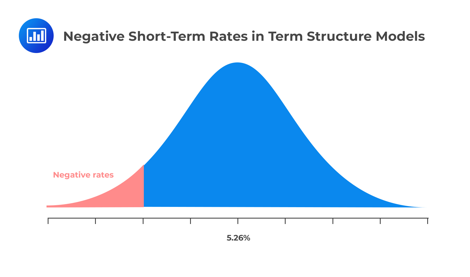
Model 1 poses a rather obvious scenario – the possibility of negative interest rates. This is, in fact, a problem with all models in which the terminal distribution of interest rates has a normal distribution. A negative interest rate makes little economic sense. It would not make much sense to lend an amount, say, $100, only to receive a smaller amount when the loan matures. In fact, an investor would be better off holding onto their cash and earning a zero rate instead.

Over a short investment horizon, say, a year, a negative rate of interest is highly unlikely. However, the possibility of a negative rate increases as the investment horizon gets longer since it is more likely that forecasted interest rates will drop below zero. For instance, consider the previous example where the annual volatility is 115 basis points. Over 10 years, for example, the standard deviation of the terminal distribution is \(1.15%×\sqrt{10}\) or 3.637%. Starting with a short-term rate of 5.26%, a random negative shock of only 5.26%/3.637% or 1.45 standard deviations would push rates below zero.

It is important to note that the problem of negative interest rates is greater when the current level of interest rates is low (e.g., 3% instead of the original 5%).

What are the Possible Solutions for Negative Interest Rates?

One of the solutions is to change the distribution of interest rates from a normal distribution to a non-negative distribution such as lognormal or chi-squared. However, a model built around a probability distribution that rules out negative rates or makes them less likely can bring about quite undesirable qualities such as skewness and inappropriate volatilities.

The other solution is to construct rate trees with the desired distribution and then simply “force” all negative rates to take a value of zero. In this approach, rates in the original tree are called the shadow rates of interest while the rates in the adjusted tree could be called the observed rates of interest. When there’s a negative rate, the observed rate takes on a value of zero until the shadow rate crosses back to a positive rate. The argument behind constraining the interest rate to positive values only is that if rates turn negative, investors have the option to hold cash.

Between the two solutions, constraining rates to positive values is more preferred because it forces a change in the original distribution only when interest rates are low. Changing the entire distribution impacts a wider range of rates.

Bottom line:

The decision of whether or not to use a model (model 1 and other normal distribution models) rests with the user. Model 1 is appropriate for the valuation of securities, such as coupon bonds, whose values mostly depend on the average path of the interest rate. For such securities, the probability of negative rates is quite low and less important. For securities that are asymmetrically sensitive to the probability of low-interest rates, however, using a normal model could be dangerous.

Term Structure Model With Drift (Model 2)

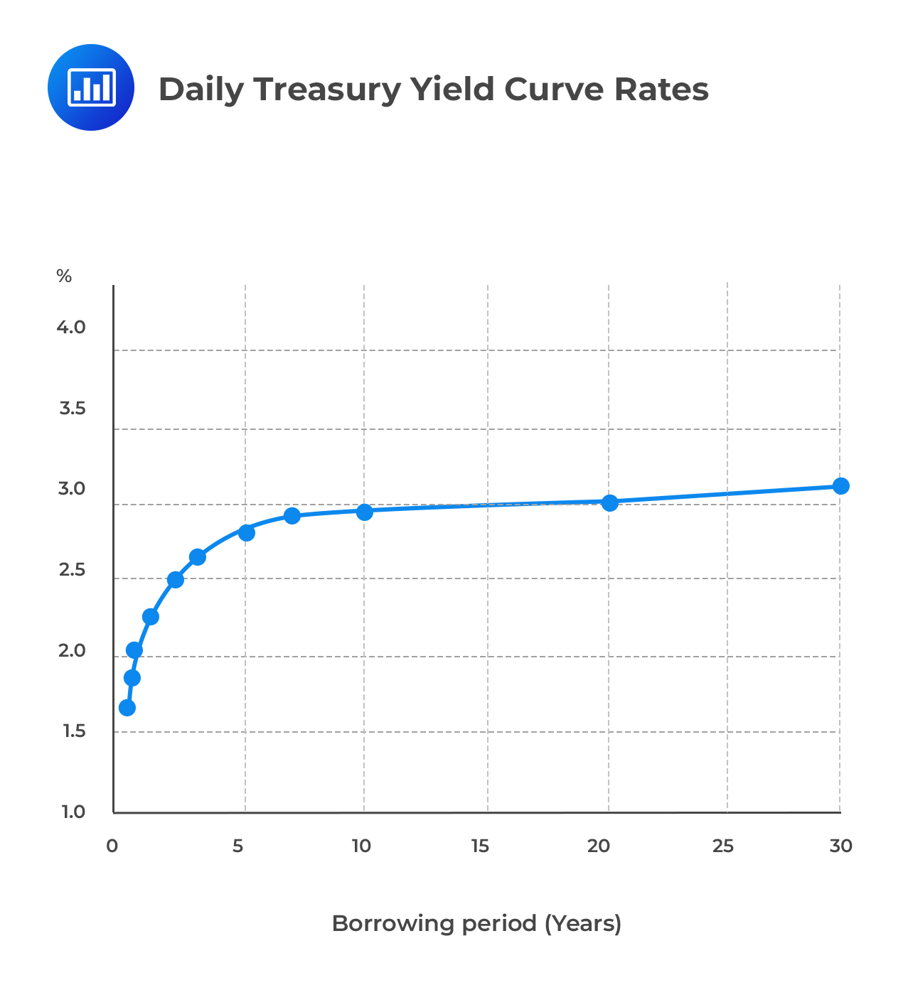
In practice, the term structure of interest rates takes on an upward sloping yield curve. This is at odds with Model 1 which assumes zero drift. The alternative is to add a positive drift term which is essentially a positive risk premium associated with longer time horizons. Under this model, the continuously compounded, instantaneous rate \(\text r_{\text t}\) is assumed to evolve according to the following equation:

$$ \text{dr}=\lambda \text{dt}+\sigma \text{dw} $$

where:

dr = Change in interest rates over a small time interval, dt.

\(\lambda\) = Drift.

dt = Small time interval (measured in years) (e.g., one month = 1/12, 2 months = 2/12, and so forth).

\(\sigma\) = Annual basis-point volatility of rate changes.

dw = Normally distributed random variable with mean 0 and standard deviation \(\sqrt{\text{dt}}\).

Example: Estimating the Change in Short-term Rate

Assume that the current value of the short-term rate is 5.26%, volatility equals 115 basis points per year, drift is 0.25%, and the time interval under consideration is one month or 1/12 years. Mathematically, \(\text r_0\) = 5.26%; \(\sigma\) = 1.15%; \(\lambda\) = 0.25%; and dt = 1/12. A month passes and the random variable, dw, with its zero mean and its standard deviation of \(\sqrt{\frac {1}{12}}\) or 0.2887, happens to take on a value of 0.25. Determine the short-term rate after one month.

Solution

The change in the short-term rate is given by:

$$ \begin{align*} \text{dr} & =\lambda \text{dt}+\sigma \text{dw} \\ &=0.25\%× \cfrac{1}{12}+1.15\%×0.25 \\ & =0.3083\% \\ \end{align*} $$

Since the short-term rate started at 5.26%, the short-term rate after a month is 5.5683%:

New short-term rate = 5.26% + 0.3083% = 5.5683%

The monthly drift is 0.25% x 1/12 = 0.0208% and the standard deviation of the rate, \(\sigma \sqrt{\text{dt}}\), is 1.15% x 0.2887 = 0.3320% (i.e., 33.2 basis points per month). The 2.08 bps drift per month (0.0208%) represents any combination of expected changes in the short-term rate (i.e., true drift) and a risk premium. For example, the drift could result from a 1.6bp change in rates coupled with a 0.48bp risk premium.

Interest Rate Tree With Drift (Model 2)

A tree over dates 0 to 2 takes the following form:

$$ \textbf{Interest Rate Tree With Drift} $$

$$ \begin{array} \hline {} & {} & {} & {\scriptsize {1/2} } & { r }_{ 0 }+2\lambda dt+2\sigma \sqrt { dt } \\ {} & {} & { \text r }_{ 0 }+\lambda \text{dt}+\sigma \sqrt { \text { dt} } & {\Huge \begin{matrix} \nearrow \\ \searrow \end{matrix} } & {} \\ { \text r }_{ 0 } & {\begin{matrix} \scriptsize {1/2} \\ \begin{matrix} \begin{matrix} \quad \quad \quad \Huge \nearrow \\ \end{matrix} \\ \quad \quad \quad \Huge \searrow \end{matrix} \\ \scriptsize {1/2} \end{matrix} } & {} & {\scriptsize \begin{matrix} \begin{matrix} {1/2} \\\scriptsize \begin{matrix} \\ \end{matrix} \end{matrix} \\ \begin{matrix} \\ \end{matrix} \\ {1/2} \end{matrix} } & {{ \text r }_{ 0 }+2 \lambda \text{dt} } \\ {} & {} & { \text r }_{ 0 }+\lambda \text{dt}-\sigma \sqrt { \text {dt} } & {\Huge \begin{matrix} \nearrow \\ \searrow \end{matrix} } & {} \\ {} & {} & {} & {\scriptsize {1/2}} & { \text r }_{ 0 }+2\lambda \text{dt}-2\sigma \sqrt { \text {dt} } \\ \end{array} $$

Note that the interest rate tree for Model 2 looks very similar to Model 1 but we add \(\lambda \text{dt}\) the drift term, which increases by \(\lambda \text{dt}\) in the next period, 2 \(\lambda \text{dt}\) in the second period, 3 \(\lambda \text{dt}\) in the third period, and so on.

Model 2 is more effective than Model 1. Intuitively, the drift term accommodates the typically observed upward-sloping nature of the term structure.

The results are satisfying in that the resulting curve can match the data much more closely than did the curve of Model 1. On the flip side, the estimated value of drift could be relatively high, especially, if considered as a risk premium only. Also, the drift can be interpreted as a combination of true drift and risk premium but this only makes practical sense in the short term. In the long-term, it is difficult to make a case for rising expected rates.

Short-term Rate Tree under the Ho-Lee Model

The Ho-Lee was introduced by Thomas Ho and Sang Bin Lee in1986. It is similar to Model 2, but with a difference: While Model 2 assumes that the drift (lambda) is constant from step to step along the tree, the Ho-Lee Model assumes that drift changes over time.

The dynamics of the risk-neutral process in the Ho-Lee model are given by:

$$ \text{dr}=\lambda_{\text t} \text{dt}+\sigma \text{dw} $$

The drift term changes from date to date. For example, there might be an annualized drift of −10 basis points in month 1, of 20 basis points in month 2, and so on.

A drift that varies with time is called a time-dependent drift.

Just as with constant drift, the time-dependent drift over each time period represents some combination of the risk premium and expected changes in the short-term rate.

The tree in the figure below illustrates the interest rate structure and effect of time-dependent drift.

$$ \textbf{Ho-Lee Model} $$

$$ \begin{array} \hline {} & {} & {} & {\scriptsize {1/2} } & { \text r }_{ 0 }+(\lambda_1 + \lambda_2) \text{dt}+2\sigma \sqrt { \text {dt} } \\ {} & {} & { \text r }_{ 0 }+\lambda_1 \text{dt}+\sigma \sqrt { \text { dt} } & {\Huge \begin{matrix} \nearrow \\ \searrow \end{matrix} } & {} \\ { \text r }_{ 0 } & {\begin{matrix} \scriptsize {1/2} \\ \begin{matrix} \begin{matrix} \quad \quad \quad \Huge \nearrow \\ \end{matrix} \\ \quad \quad \quad \Huge \searrow \end{matrix} \\ \scriptsize {1/2} \end{matrix} } & {} & {\scriptsize \begin{matrix} \begin{matrix} {1/2} \\\scriptsize \begin{matrix} \\ \end{matrix} \end{matrix} \\ \begin{matrix} \\ \end{matrix} \\ {1/2} \end{matrix} } & { \text r }_{ 0 }+(\lambda_1 + \lambda_2) \text{dt} \\ {} & {} & { \text r }_{ 0 }+\lambda_1 \text{dt}-\sigma \sqrt { \text {dt} } & {\Huge \begin{matrix} \nearrow \\ \searrow \end{matrix} } & {} \\ {} & {} & {} & {\scriptsize {1/2}} & { \text r }_{ 0 }+(\lambda_1 + \lambda_2) \text{dt}-2\sigma \sqrt { \text {dt} } \\ \end{array} $$

\(\lambda_1\) and \(\lambda_2\) are estimated from observed market prices.

For each period, drift for the first period is the observed spot interest rate. Drift for the second period is estimated from the market price of two-period securities and the first-period drift.

Drift for the third period is calibrated from the first-period rate, drift of the second year, and the market price of three-period securities.

Uses and Benefits of Arbitrage-free Models

In broad terms, there are two types of models: arbitrage-free models and equilibrium models. The key issue in choosing between the two types is the desirability of fitting the model to match market prices. This choice depends on the purpose of the model.

Arbitrage-free short-rate models are used to generate the true stochastic interest rate generating process by using real market data. They are particularly appropriate for quoting the prices of securities that do not have an active market traded based on the prices of more liquid securities.

To see how this works, consider a customer interested in an odd maturity swap with a term of say, four years and five months. If the customer asks for a quote, the swap desk would not be able to fetch the quote directly from the market because a liquid market for a swap of that particular duration is likely to be unavailable. Liquid market prices might be observable only for three- and five-year swaps, or – as is common – for two- and five-year swaps. In this situation, the swap desk may price the odd-maturity swap using an arbitrage-free model essentially as a means of interpolating between observed market prices.

Arbitrage-free models are also used to value and hedge derivative securities for the purpose of making markets or for proprietary trading. For example, the observable price of a bond can be used to price an option on the bond.

Fitting models to market prices is informed by the argument that market prices reflect a good deal of information about the future behavior of interest rates, and, therefore, a model fitted to those prices captures that interest rate behavior.

Be that as it may, there are two caveats:

1. A mediocre model cannot be rescued by calibrating it to match market prices. If, for example, the parallel shift assumption is not appropriate, adding a time-dependent drift to create a better fitting model will not make the model any more suitable for that application.
2. Arbitrage models assume that the underlying prices are accurate but this will not be the case if there is an external, temporary, exogenous shock.

For instance, a glut in the supply of a security resulting from forced liquidation which potentially drives down the market price.

Equilibrium short rate models are based on the laws of economics such as supply-demand and require knowledge of investor preferences and probabilities. Unlike arbitrage-free short rate models, equilibrium short rate models make certain assumptions about the true interest rate generating process to determine the correct theoretical term structure. They are appropriate for relative analysis (i.e., comparing the values of two securities). This is particularly because they do not require the constraint that the underlying securities are priced accurately. Arbitrage-free models are not appropriate for such an exercise because they assume that both securities are correctly/properly priced.

The Process of Constructing a Simple and Recombining Tree for a Short-term Rate under the Vasicek Model With Mean Reversion

The Vasicek Model introduces mean reversion into the rate model. The model is based on the premise that short-term interest rates exhibit mean reversion and that there’s some sort of a long-term equilibrium:

• When the short-term rate is below its long-run equilibrium value, the drift is positive, driving the rate up toward a long-run value.
• When the rate is above its equilibrium value, the drift is negative, driving the rate up toward this equilibrium value.

The Vasicek model is given by:

$$ \text{dr}=\text k(\theta-\text r)\text{dt}+\sigma \text{dw} $$

where:

k = A parameter that measures the speed of reversion adjustment.

\(\theta\) = Long-run value of the short-term rate assuming risk neutrality.

r = Current interest rate level.

A high k will produce quicker (larger) adjustments than smaller values of k. Furthermore, the greater the difference between r and \(\theta\), the greater the expected change in the short-term rate toward \(\theta\).

Just as with model 2, the drift term, \(\lambda\), is a combination of the expected rate change and a risk premium. Under the assumption of risk-neutrality, the long-run value of the short-term rate can be approximated as:

$$ \theta \approx {\text r}_l+\cfrac {\lambda}{\text k} $$

where \(\text r_{\text l}\) is the long-run true rate of interest.

Example: Long-run Value of Short-term Rate under the Vasicek Model

Consider a Vasicek model with a reversion adjustment parameter of 0.05, an annual standard deviation of 130 basis points, a true long-term interest rate of 5%, a current interest rate of 6.0%, and an annual drift of 0.40%. Determine the forecasted change in the short term rate for the next period.

Solution

First, we have to determine \(\theta\), the long-run value of the short-term rate assuming risk neutrality:

$$ \theta \approx {\text r}_{\text l}+\cfrac {\lambda}{\text k}\approx 5\%+\cfrac {0.40\%}{0.05}=13\% $$

It follows that the forecasted change in the short-term rate for the next period is 0.0292%:

$$ \begin{align*} \text{dr} & =\text k(\theta -{\text r}){\text {dt}} \\ & =0.05(13\%-6\%)\left(\cfrac {1}{12} \right)=0.0292\% \\ \end{align*} $$

The volatility for the monthly interval is computed as \(1.3\% \times \sqrt{\cfrac {1}{12}} = 0.38\%\) (38 basis points per month).

Representing this process with a tree is not quite as straightforward as the simpler processes we have looked at previously. Particularly, this is because it leads to a non-recombining tree. The tree fails to recombine because the adjustment in time 2 after a downward movement in interest rates will be larger than the adjustment in time 2 following an upward movement in interest rates (since the lower node rate is further from the long-run value). Let’s demonstrate the process assuming a starting rate of 6%.

$$ \textbf{Vasicek Model Data} $$

$$ \begin{array}{l|c} \text{Initial short rate} & {6.0\%} \\ \hline \text{dt (month)} & {0.0833} \\\hline \text{Drift, annual} & {0.4\%} \\\hline \text{Drift, per month} & {0.0333\%} \\\hline \text{Volatility, annual} & {1.3\%} \\\hline {\text{Theta}, \theta} & {13\%} \\\hline {\text K} & {0.05} \\ \end{array} $$

$$ \textbf{First Period Upper and Lower Node Calculations} $$

$$ \bf{\text{dr}=\text k(\theta – \text r){\text {dt}}+ \sigma \text{dw}} $$

$$ \textbf{Calculation} $$

$$ \begin{array} \hline {} & {\small \frac { 1 }{ 2 } } & {6.4045\%} & {{\Huge \longrightarrow} {6.0\% + 0.05 \left(13\%-6\%\right) \frac {1}{12}+ \frac{1.3\%}{\sqrt{12}} }} \\ 6.0\% & {\Huge \begin{matrix} \nearrow \\ \searrow \end{matrix} } & {} & {} \\ {} & {\small \frac { 1 }{ 2 }} & {5.6539\%} & {{\Huge \longrightarrow} {6.0\% + 0.05 \left(13\%-6\%\right) \frac {1}{12}- \frac{1.3\%}{\sqrt{12}} } } \\ \end{array} $$

If the interest rate evolves upward in the first period, we would turn to the upper node in the second period. The interest rate process can move up to 6.8073% or down to 6.0567%.

$$ \textbf{Second Period Upper Node Calculations} $$

$$ \bf{\text{dr}=\text k(\theta – \text r){\text {dt}}+ \sigma \text{dw}} $$

$$ \textbf{Calculation} $$

$$ \begin{array} \hline {} & {\small \frac { 1 }{ 2 } } & {6.8073\%} & {{\Huge \longrightarrow} {6.4045\% + 0.05 \left(13\%-6.4045\%\right) \frac {1}{12}+ \frac{1.3\%}{\sqrt{12}} }} \\ 6.4045\% & {\Huge \begin{matrix} \nearrow \\ \searrow \end{matrix} } & {} & {} \\ {} & {\small \frac { 1 }{ 2 }} & {6.0567\%} & {{\Huge \longrightarrow} {6.4045\% + 0.05 \left(13\%-6.4045\%\right) \frac {1}{12}- \frac{1.3\%}{\sqrt{12}} }} \\ \end{array} $$

If the interest evolves downward in the first period, we would turn to the lower node in the second period. The interest rate process can move up to 6.0598% or down to 5.3092%.

$$ \textbf{Second Period Lower Node Calculations} $$

$$ \bf{\text{dr}=\text k(\theta – \text r){\text {dt}}+ \sigma \text{dw}} $$

$$ \textbf{Calculation} $$

$$ \begin{array} \hline {} & {\small \frac { 1 }{ 2 } } & {6.0598\%} & {{\Huge \longrightarrow} {5.6539\% + 0.05 \left(13\%-5.6539\%\right) \frac {1}{12}+ \frac{1.3\%}{\sqrt{12}} }} \\ 5.6539\% & {\Huge \begin{matrix} \nearrow \\ \searrow \end{matrix} } & {} & {} \\ {} & {\small \frac { 1 }{ 2 }} & {5.3092\%} & {{\Huge \longrightarrow} {5.6539\% + 0.05 \left(13\%-5.6539\%\right) \frac {1}{12}- \frac{1.3\%}{\sqrt{12}} }} \\ \end{array} $$

Finally, we can combine all the nodes to come up with the following non-recombining tree:

$$ \textbf{2-Period Interest Rate (Non-combining) Tree with Mean Reversion} $$

$$ \begin{array} {} & {} & {\small \scriptsize { {1/2}} } & 6.8073\% \\ {} & 6.4045\% & {\Huge \begin{matrix} \nearrow \\ \searrow \end{matrix} } & {} \\ 6.0\% \begin{matrix} & {\small \scriptsize { {1/2}} } & \\ &\Huge \nearrow & \\ &\Huge \searrow & \\ & {\small \scriptsize { {1/2}} } & \end{matrix} & {} & \begin{matrix} {\small \scriptsize { {1/2}} } \\ \\ {\small \scriptsize { {1/2}} } \end{matrix} & \begin{matrix} 6.0567\% \\ \\ 6.0598\% \end{matrix} \\ {} & 5.6539\% & {\Huge \begin{matrix} \nearrow \\ \searrow \end{matrix} } & {} \\ {} & {} & {\small \scriptsize { {1/2}} } & 5.3092\% \\ \end{array} $$

As observed, the Vasicek model has generated a 2-period non-recombining tree of short-term interest rates. However, it is possible to come up with adjustments so that a recombining tree is the end result.

Step 1: Find the average of the two middle nodes.

$$ \text{Average} = \cfrac {6.0567\% + 6.0598\%}{2} = 6.0583\% $$

Step 2: Do away with the 50% probability of up-down movements and replace them with (p, 1 — p) and (q, 1 — q). This has been demonstrated below:

$$ \textbf{Recombining the Interest Rate Tree} $$

$$ \begin{array} \hline {} & {} & {} & {\scriptsize {\text p} } & { \text r^{\text{uu}} } \\ {} & {} & { 6.4045\% } & {\Huge \begin{matrix} \nearrow \\ \searrow \end{matrix} } & {} \\ { 6.0\% } & {\begin{matrix} \scriptsize {1/2} \\ \begin{matrix} \begin{matrix} \quad \quad \quad \Huge \nearrow \\ \end{matrix} \\ \quad \quad \quad \Huge \searrow \end{matrix} \\ \scriptsize {1/2} \end{matrix} } & {} & {\scriptsize \begin{matrix} \begin{matrix} {1-\text p} \\\scriptsize \begin{matrix} \\ \end{matrix} \end{matrix} \\ \begin{matrix} \\ \end{matrix} \\ {\text q} \end{matrix} } & { 6.0583\% } \\ {} & {} & { 5.6539\% } & {\Huge \begin{matrix} \nearrow \\ \searrow \end{matrix} } & {} \\ {} & {} & {} & {\scriptsize {1-\text q}} & { \text r^{\text{dd}} } \\ \end{array} $$

Step 3: Solve for p, q, \({ \text r^{\text{uu}} }\), and \({ \text r^{\text{dd}} }\).

P and q are the respective probabilities of up movements in the trees in the second period after the up and down movements in the first period. 1 – P and 1 – q are the respective probabilities of down movements in the trees in the second period after the up and down movements in the first period. ruu and rdd are the respective interest rates from successive (up, up and down, down) movements in the tree.

According to the general formula for the risk-neutral Vasicek process, i.e., \( {\text{dr}=\text k(\theta – \text r){\text {dt}}+ \sigma \text{dw}} \), and the parameter values set in this section, the expected rate and standard deviation of the rate from 6.4045% are, respectively,

$$ 6.4045\%+0.05(13\%-6.4045\%)\cfrac {1}{12}=6.4320\% $$

And

$$ \cfrac {1.3\%}{\sqrt{12}}=0.3753\% $$

For the recombining tree to match this expectation and standard deviation, it must be the case that:

\(p×\text r^{\text{uu}}+(1-\text p)×6.0583\%=6.4320\% \) …………………..equation 1

and, by the definition of standard deviation,

\(\sqrt{[\text p(\text r^{\text{uu}}-6.4320\%)^2+(1-\text p) (6.0583\%-6.4320\%)^2 ] }=0.3753\%\)…equation 2

Solving equations 1 and 2 would give us the values of \(\text r^{\text{uu}}\) and p.

We would then repeat the process for the bottom portion of the tree, solving for q and \(\text r^{\text{dd}}\).

Calculating the Vasicek Model Rate Change, Standard Deviation of the Rate Change, Expected Rate in T years, and Half-Life

In this section, we turn our attention to the process of mean reversion starting at a specified current rate.

The expectation or mean of the short-term rate as a function of horizon gradually rises from its current value toward its limiting value of \(\theta\) – the long-run value of the short-term rate assuming risk neutrality. For example, given a current value of 6.0%, a long-run value of 13% with the mean-reversion parameter, k, of 0.05, the long-term mean-reverting level will eventually reach 13%. It will, however, take a long time since the value of k is quite small. The difference between the current value and the long-run value, i.e., 7%, decays exponentially at the rate of mean reversion.

To forecast the rate in 10 years, we note that \(7\%× \text {exp}^{-0.05×10}=4.2457\%\).

Therefore, the expected rate in 10 years is \(13\% – 4.2457\% = 8.7543\%\).

For completeness, the expectation of the rate in the Vasicek model after.

T years is given by:

$$ \text r_{0} {\text e}^{-\text{kT}}+\theta (1-\text e^{-\text{kT}} ) $$

In words, the expectation is a weighted average of the current short rate and its long-run value, where the weight on the current short rate decays exponentially at a speed determined by the mean-reverting parameter.

Example: Expected Rate in Vasicek Model after T Years

Consider a Vasicek model with a reversion adjustment parameter of 0.03, annual standard deviation of 200 basis points, a true long-term interest rate of 6%, a current interest rate of 5.0%, and annual drift of 0.35%. Determine the expected rate in the model after 10 years:

Solution

The expectation of the rate in the Vasicek model after T years is given by:

$$ \text r_{0} {\text e}^{-\text{kT}}+\theta (1-\text e^{-\text{kT}} ) $$

Where:

\(\text r_{0}\) = Current interest rate.

K = Mean reversion parameter.

\(\theta\) = Long-run value of the short-term rate assuming risk neutrality.

T = Time in years.

First, we must work out the value of \(\theta\)

$$ \theta \approx {\text r}_{\text l}+\cfrac {\lambda}{\text k}\approx 6\%+\cfrac {0.35\%}{0.03}=17.67\% $$

\({\text r}_{\text l}\) is true long-term interest rate, and \(\lambda\) is the annual drift

Therefore,

$$ \begin{align*} \text{the expected rate after 10 years } & = 5\% {\text e}^{-0.03×10}+17.67\%(1-{\text e}^{-0.03×10} ) \\ & =3.7041\% + 4.5797\% \\ &= 8.2838\% \\ \end{align*} $$

Half-life

The mean-reverting parameter k does not intuitively describe the pace of mean-reversion. A more intuitive quantity is the factor’s half-life, defined as the time it takes the factor to progress half the distance toward its goal. The half-life is given by:

$$ \text{Half-life} =\tau_{\text{years}}=\cfrac {\text{ln}⁡(2)}{\text k} $$

In the previous example where k = 0.03, the half-life is 23.1 years [= ln(2)/0.03].

In words, the interest rate factor takes 23.1 years to cover half the distance between its starting value and its goal.

A larger mean reversion adjustment parameter results in a shorter half-life.

Effectiveness of the Vasicek Model

The mean reversion parameter under the Vasicek model not only improves the specification of the term structure but also produces a specific term structure of volatility. Specifically, the Vasicek model will produce a term structure of volatility that is declining. This is particularly true when we consider that the development of the mean-reverting model, the parameters r0 and θ are calibrated to match observed market prices. As a result, the Vasicek model produces a term structure of volatility that is declining, implying that it overstates short-term volatility but understates long-term volatility. In contrast, Model 1 which has zero drift generates a flat volatility of interest rates across all maturities.

Mean reversion in the Vasicek model also has implications on long-lived and short-lived economic news. Economic news is said to be long-lived if it changes the market’s view of the economy many years in the future. A good example would be the emergence of game-changing AI technology that raises productivity, triggering a long-lived shock to the system. Economic news is said to be short-lived if it changes the market’s view of the economy strictly in the near future. A good example would be a decline in retails sales attributable to excessively cold weather over the holiday season.

• A very low mean reversion parameter, i.e., a very long half-life, implies that news is long-lived and that it will affect the short rate for many years to come.
• A very high mean reversion parameter, i.e., a very short half-life, implies that news is short-lived and that it affects the short rate for a relatively short period of time.

Question 1

Assume that we are provided with a set of data whose current short-term rate of 3.02% has a volatility of 103 basis points per year. We are also given a constant \(\lambda \) whose value is 0.225%. Using the model of drift and risk premium, compute the change in rate if the monthly realization of the random variable \(dw\) is 0.24.

1. 0.0050%.
2. 0.2660%.
3. 0.0212%.
4. 0.0027%.

The correct answer is B.

From model 2 (drift and risk premium model), we have:

$$ dr=\lambda dt+\sigma dw $$

We are given:

\(\lambda=0.225\%\).

\({ r }_{ 0 }=3.02\%\).

\(\sigma =1.03\%\).

\(dw=0.24\).

The time interval under consideration is one month or \(\frac { 1 }{ 12 } \) years.

Hence:

$$\begin{align*} dr&=0.225\%\times \frac { 1 }{ 12 } +1.03\%\times 0.24\\ & \Rightarrow dr=0.266\% \end{align*}$$

Question 2

We are given the following for the Vasicek model:

$$ \begin{align*}dr&=k\left( { r }_{ \infty }-r \right) dt+\lambda dt+\sigma dw\\ & =k\left( \left[ { r }_{ \infty }+\frac { \lambda }{ k } \right] -r \right) dt+\sigma dw \end{align*}$$

The speed of mean reversion is 0.63, and the true interest rate process exhibits mean reversion to a long-term value, \({ r }_{ \infty }\), of \(6.3\%\). Further, the current short term rate is \(5.2\%\) and \(\sigma=3.1\%\). Using the model provided, determine the expected change in the short rate and the volatility over the next month consecutively if \(\lambda=0.3\%\).

1. 69.3 basis points.
2. 9.2 basis points.
3. 8.3 basis points.
4. 5.8 basis points.

The correct answer is C.

From the above information, we have that:

\(k=0.63\).

\({ r }_{ \infty }=6.3\%\).

\( \sigma=3.1\%\).

\({ r }_{ 0 }=5.2\%\).

\(\lambda=0.256\%\).

Thus, the expected change in the short rate is:

$$ \begin{align*} dr&=k\left( \theta -r \right) dt+\sigma dt\\ & =k\left( \left[ { r }_{ \infty }+\frac { \lambda }{ k } \right] -r \right) dt+\sigma dw\end{align*} $$

Remember that:

$$\begin{align*} \theta &\equiv { r }_{ \infty }+\frac { \lambda }{ k }\\ \therefore \theta& \equiv 6.3\%+\frac { 0.3\% }{ 0.63 } =6.78\%\\ &=0.63\times \left( 6.78\%-5.2\% \right) \frac { 1 }{ 12 } =0.0008295\text{ or} 8.295\text{ basis points}\end{align*} $$

Question 3

A dataset has a mean-reverting parameter of 0.22 and a volatility of 103 basis points. If the short-term rate is normally distributed, then use the Vasicek model to determine the standard deviation of the terminal distribution of the short rate after 2 years.

1. 0.0119.
2. 0.0001.
3. 0.0168.
4. 0.0093.

The correct answer is A.

Remember that the standard deviation of the terminal distribution of the short rate after \(T\) years is:

$$ \sqrt { \frac { { \sigma }^{ 2 }\left( 1-{ e }^{ -2kT } \right) }{ 2k } } $$

Therefore:

$$ \sqrt { \frac { { 0.0103 }^{ 2 }\left( 1-{ e }^{ -2\times 0.22\times 2 } \right) }{ 2\times 0.22 } } =0.0119 $$