Study Materials for 2023 CFA®, FRM®, Actuarial, GMAT® and EA® Exams

SOA Exam FM Study Notes

Online and Printable Prep Books for Actuarial Exam FM

Exam FM is a three-hour, 35 multiple-choice questions exam designed to test your knowledge of fundamental concepts of financial mathematics. AnalystPrep has developped concise study notes focusing on exactly the learning objectives tested in the Society of Actuaries exams.

SOA Exam FM’s syllabus comprises of 8 topics and each one of them contributes a certain percentage of questions to the exam. With AnalystPrep’s concise study notes for Exam FM, you can simply read on your tablet, computer, or print each concept before jumping into the question bank portion of the platform.

4.5  Million
Questions Answered by our Users
50  Thousand
Satisfied Customers
# 1  Rated
Preparation Platform By Review Websites
Wave Wave
soa-fm-notes-2

What are the Eight Topics?

The first fours topics are quite straightforward and most actuarial students should have seen the most part of this in their undergraduate degree:

  • Time value of money (10-15%)
  • Annuities/cash flows with non-contingent payments (15-20%)
  • Loans (10-20%)
  • Bonds (10-20%)

The next two topics relate mostly to the investment world and can be a little more tricky for actuarial students:

  • General cash flows and portfolios (15-20%)
  • Immunization (10-15%)

And the last two topics are based on interest rate and interest rate theory, but weight a bit less on the overall exam:

  • Interest rate swaps (0-10%)
  • Determinants of interest rates (0-10%)

Here, it is important to note that having great fundamentals in the first few topics will help you solve more easily questions from the later topics.

How Should I Study for Exam FM?

To improve your chances of passing Exam FM:

Financial Mathematics Notes

Start off by reading the study notes. These are based exactly on the learning objectives that the SOA tests and are accompanied by relevant examples to illustrate each concept.

Improve your Performance

Our question bank is divided into topics so that you can concentrate on each particular area. As you get closer to the exam, you can then mix those topics together and even create an FM practice exam using our Quiz function.
soa-fm-question-bank

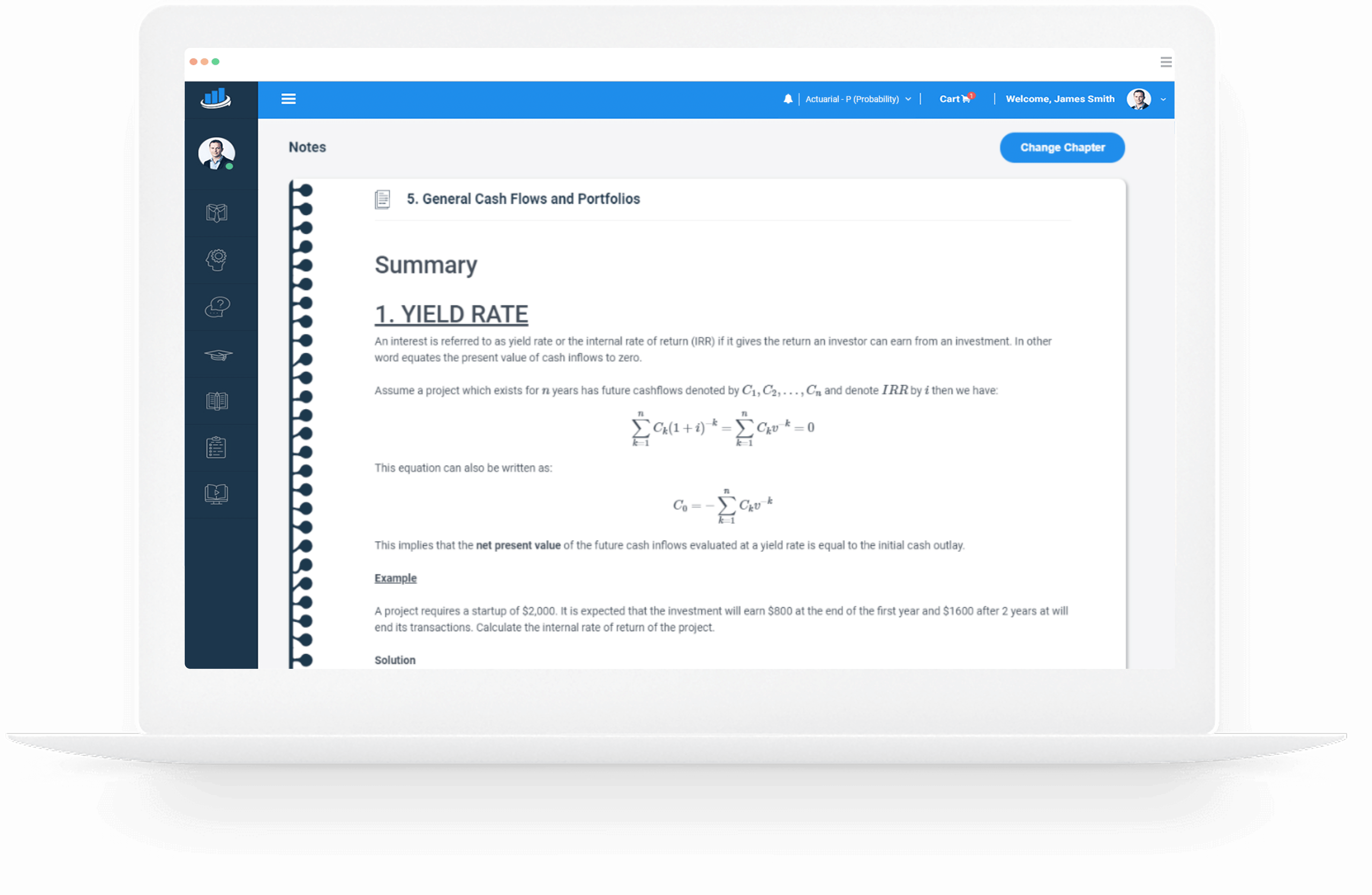
Example Learning Objective from AnalystPrep's SOA Exam P Prep Notes

Topic 2: Loans

Summary

A loan can be considered a compound interest transaction where the amount borrowed (Principal) is paid by regular payments at a fixed rate of interest, for a predetermined period(term of the loan). The payment of the loan can sometimes involve drop payment, which is a short term payment made at the end of the loan term.

Individuals or companies raise their funds by taking loans from financial providers such as banks.

Let \(L\) bet the amount of the loan to be paid \(n\) installments of \(X\) and the rate of interest \(i\) at the end of each period. Then the equation of value will be:$$
X{ a }_{ \overline { n| } }=L $$
As an eye-opener, consider the following example.

Example 1

A cooperative society lends a farmer $1000 which is supposed to be paid at the end of each year for 3 years. The interest rate charged on the loan is 10%.

Calculate the amount of each annual payment.

  1. 309.45
  2. 408.56
  3. 305.45
  4. 234.78
  5. 402.11

Solution

The correct answer is E

let the annual payments be $X. Then the equation of value is:
$$ X{ a }_{ \overline { 3 } | }=1000\Rightarrow X=\frac { 1000 }{ { a }_{ \overline { 3 } | } } =\frac { 1000 }{ 2.486852 } =402.1148 $$
Therefore, the farmer pays 402.1148 at the end of the first, second and third year. It is important to note that this amount covers the interest and capital repayment parts of the loan.

Consider the example 1 above:

The initial capital amount of money is $1000. The first payment of the loan is at time 1 and the interest due is \(0.1\times 1000=$100\). This is the interest part of the payment 402.1148 so the capital repayment is \(402.1148-100=302.1148\) . Therefore, the capital outstanding just after the first payment is \(1000-302.1148=697.8852\).

At the second year, the interesting part will be \(0.1 \times 697.8852=69.78852\). The capital repayment part is \(402.1148-69.78852=332.32628\) . So, the outstanding capital after the second payment is \(697.8852-332.32628=365.559\)

At the end of the loan term, the interest due will be \(0.1\times365.55892=36.555892\). So, the capital repayment is \(402.1148-36.555892=365.559\) and thus the capital is exactly at the last payment.

The above example should set a way of knowing how loans are transacted. It is worth to note that knowledge from the annuities is important here.

Calculating the Loan Balance(Capital Outstanding)

Consider the transaction of a loan at time n which the end of the loan term. That is the last payments of the loan exactly covers the capital outstanding and the interest due. Now, let

\({ L }_{ k }\) – the amount of the loan outstanding at any time k=0,1,2,…n

\({ X }_{ k }\) – regular installments paid at any time \(k=1,2,\cdots n\)

\({ C }_{ k }\) -the capital repaid at time \(k=1,2,\cdots n\)

\({ I }_{ k }\) -interest amount paid at time \(k=1,2,\cdots n\)

\(i\)- interest rate charged on the loan

The at any time \(k=1,2,\cdots n ,\)
$$ { X }_{ k }={ L }_{ k }+{ I }_{ k } $$
And the equation of value is given by:
$$ { L }_{ 0 }={ X }_{ 1 }v+{ X }_{ 2 }{ v }^{ 2 }+\cdot \cdot \cdot +{ X }_{ n }{ v }^{ n } $$
Which is clearly intuitive

Note also that:
$$ { I }_{ k }=i{ L }_{ k-1 } \quad and \quad { C }_{ k }={ L }_{ k-1 } $$
From the last result, it is easy to see that:
$$ { X }_{ k }=i{ L }_{ k-1 }+{ L }_{ k-1 } $$
You can refer to example 1 and see how these formulas can be applied.

There are two methods in calculating the Loan Balance:

    1. The Prospective Method


    1. The Retrospective Method


The Prospective method.

This method calculates the loan balance as the sum of the present value of the future payments that will be made at a given interest rate within the term of the loan.
We know that:
$$ { I }_{ k }={ iL }_{ k-1 } $$
And
$$ { C }_{ k }={ L }_{ k-1 } $$
So that,
$$ \begin{align*}
{ X }_{ k } &={ I }_{ k }+{ C }_{ k }={ iL }_{ k-1 }+{ L }_{ k-1 }\quad so,\\ { X }_{ k } &={ iL }_{ k-1 }+{ L }_{ k-1 }\quad \\ & =\left( 1+i \right) { L }_{ k-1 }\\ \Rightarrow { L }_{ k-1 } &=v{ X }_{ k }
\end{align*}$$
From the last expression, it is easy to see that the capital outstanding at time \(k-1\) is equivalent to the present value of the future payment at time \(k\).

From the above result, we are comfortable to see that, at any time \(k=1,2,…n\) ,
$$ \begin{align*}
{ L }_{ k } &={ X }_{ k+{ 1 } }v+{ X }_{ k+{ 2 } }{ v }^{ 2 }+{ X }_{ k+{ 3 } }{ v }^{ 3 }+\cdot \cdot \cdot +{ X }_{ n }{ v }^{ { n-k } }\\ &=X{ a }_{ \overline { n-k } | }\quad (Note\quad that\quad we\quad assume\quad that\quad the\quad annual\quad payment\quad is\quad constant)
\end{align*}$$
Which completes the definition of the prospective method of calculating the loan balance.

Example 2

A cooperative society lends a farmer $1000 which is supposed to be paid at the end of each year for 3 years. The interest rate charged on the loan is 10%.

Calculate the capital outstanding after the first payment using the prospective method.

  1. 697.88
  2. 600.97
  3. 778.89
  4. 765.43
  5. 765.34

Solution

The correct answer is A.

let the annual payments be $X. Then the equation of value is:
$$ X{ a }_{ \overline { 3 } | }=1000\Rightarrow X=\frac { 1000 }{ { a }_{ \overline { 3 } | } } =\frac { 1000 }{ 2.486852 } =402.1148 $$
We know that:
$$ { L }_{ k }={ X }_{ k+{ 1 } }v+{ X }_{ k+{ 2 } }{ v }^{ 2 }+{ X }_{ k+{ 3 } }{ v }^{ 3 }+\cdot \cdot \cdot +{ X }_{ n }{ v }^{ { n-k } } $$
We need:
$$ { L }_{ 1 }={ X }_{ 2 }v+{ X }_{ 3 }{ v }^{ 2 }=402.1148{ \left( 1.1 \right) }^{ -1 }+402.1148{ \left( 1.1 \right) }^{ -2 }=697.8852 $$
So,
$$ { L }_{ 1 }=697.8852 $$
Retrospective Approach

This approach can be described as “backward-looking”. It computes the capital outstanding as the accumulated amount of the loan at the time of valuation less the accumulated value of all regular payments (installments) that has been paid up to the time of valuation.

Using the same notation defined above we know that:
$$ { I }_{ k }={ iL }_{ k-1 } $$
So that:
$$ { I }_{ 1 }={ iL }_{ 0 } $$
We also know that:
$$ \begin{align*}
{ X }_{ k }&={ iL }_{ k-1 }+{ C }_{ k }\\ \Rightarrow { C }_{ k }&={ X }_{ k }-{ iL }_{ k-1 }\quad \left( Recall\quad that\quad { C }_{ k }={ L }_{ k-1 } \right)
\end{align*}$$
So that the capital repaid at time k=1 is:
$$ { C }_{ 1 }={ X }_{ 1 }-{ iL }_{ 0 } $$
So the loan balance after the first payment will be:
$$ \begin{align*}
{ L }_{ 1 }&={ L }_{ 0 }-\left( { X }_{ 1 }-{ iL }_{ 0 } \right) \\ \\& ={ L }_{ 0 }\left( 1+i \right) -{ X }_{ 1 }
\end{align*}$$
Intuitively, at any time \(k\ge 1\) the interest due at that point will be:
$$ { I }_{ k }={ iL }_{ k-1 } $$
And the capital repaid is:
$$ { C }_{ k }={ X }_{ k }-{ iL }_{ k-1 } $$
So, the loan balance at any time k will be:
$$ { L }_{ k }={ L }_{ k-1 }\left( 1+i \right) -{ X }_{ k } $$
At this point, it is easy to see that, if we work from time k to time 0,
$$ { L }_{ k }={ L }_{ 0 }{ \left( 1+i \right) }^{ k }-\left[ { X }_{ 1 }{ \left( 1+i \right) }^{ k-1 }+{ X }_{ 2 }{ \left( 1+i \right) }^{ k-1 }+\cdot \cdot \cdot +{ X }_{ k-1 }{ \left( 1+i \right) }+{ X }_{ k } \right] $$
So,
$$ { L }_{ k }={ L }_{ 0 }{ \left( 1+i \right) }^{ k }-X{ s }_{ \overline { k } | } $$
Which completes the definition of calculating loan balances using the retrospective method.

Example 3

A cooperative society lends a farmer $1000 which is supposed to be paid at the end of each year for 3 years. The interest rate charged on the loan is 10%.

Calculate the capital outstanding after the first payment using the retrospective method.

  1. 675.43
  2. 697.89
  3. 700.56
  4. 765.43
  5. 800.45

Solution

The correct answer is B
$$ { L }_{ k }={ L }_{ 0 }{ \left( 1+i \right) }^{ k }-\left[ { X }_{ 1 }{ \left( 1+i \right) }^{ k-1 }+{ X }_{ 2 }{ \left( 1+i \right) }^{ k-1 }+\cdot \cdot \cdot +{ X }_{ k-1 }{ \left( 1+i \right) }+{ X }_{ k } \right] $$
This can be written as:
$$ { L }_{ k }={ L }_{ 0 }{ \left( 1+i \right) }^{ k }-X{ s }_{ \overline { k } | } $$
We need:
$$ { L }_{ 1 }={ L }_{ 0 }{ \left( 1+i \right) }^{ 1 }-X{ s }_{ \overline { 1 } | } $$
Now,

let the annual payments be $\(X\). Then the equation of value is:
$$ \begin{align*}
X{ a }_{ \overline { 3 } | }&=1000\Rightarrow X=\frac { 1000 }{ { a }_{ \overline { 3 } | } } =\frac { 1000 }{ 2.486852 } =402.1148 \\ \Rightarrow { L }_{ 1 }&=1000{ \left( 1.1 \right) }^{ 1 }-402.1148{ \left( 1 \right) } \\& =1100-402.1148=697.885
\end{align*}$$
It is easy to show that both methods lead to the same result. The retrospective method is given by:
$$ \begin{align*}
{ L }_{ 0 }{ \left( 1+i \right) }^{ k }-X{ s }_{ \overline { k } | } &=X{ a }_{ \overline { n } | }{ \left( 1+i \right) }^{ k }-X{ s }_{ \overline { k } | }\left( since\quad { L }_{ 0 }={ a }_{ \overline { n } | } \right) \\ &=X\left[ \frac { 1-{ v }^{ n } }{ i } { \left( 1+i \right) }^{ k }-\frac { { \left( 1+i \right) }^{ k }-1 }{ i } \right] \quad (Apply \quad simple \quad Algebra ) \\ &=X\left[ \frac { 1-{ v }^{ n-k } }{ i } \right] \\ &=X{ a }_{ \overline { n-k } | }@i
\end{align*}$$
The last expression is simply the formula for calculating the loan balance prospectively. So,
$$ { L }_{ 0 }{ \left( 1+i \right) }^{ k }-X{ s }_{ \overline { k } | }=X{ a }_{ \overline { n-k } | }@i $$
Calculating the Interest due and Loan balance at any time.

From the formula, \({ I }_{ k }={ iL }_{ k-1 }\) , it is easy to see that after finding capital outstanding, we can find the capital element of each installment.

Consider the following example 3 above:

Assume that we want to find interest due just after the first payment. We had calculated the capital outstanding to be 697.885

So,
$$ \begin{align*}
{ I }_{ k }&={ iL }_{ k-1 } \\ &=0.1\times 697.885=69.7885
\end{align*}$$
Generally, the interest payment is gotten by calculating the loan balance after the previous payment and then the interest by multiplying by the interest by multiplying the effective rate of interest and the previous capital outstanding. The capital element of an installment is gotten by subtracting the interest from the installment.

Example 4

An investor takes a loan of $32000 from a bank which is repaid by 10 equal payments made at the end of each year. The effective rate of interest is 4%.

Calculate the interest due to the 4th payment.

  1. 947.2
  2. 958.67
  3. 897.2
  4. 654.32
  5. 567.56

Solution

The correct answer is A

Let the annual payment be $\(X\). So,
$$ X{ a }_{ \overline { 10 } | }=32000\Rightarrow X=\frac { 32000 }{ { a }_{ \overline { 10 } | } } =\frac { 32000 }{ 8.110896 } =3945.3102 $$
We need to find the loan balance after the 3rd payment. That is:
$$ \begin{align*}
{ L }_{ k }&=X{ a }_{ \overline { n-k } | }\\ \Rightarrow { L }_{ 3 }&=X{ a }_{ \overline { 7 } | }\\ &=3945.3102\times 6.0021=23679.9675
\end{align*}$$
So, the interest element of the 4th element is:
$$ \begin{align*}
{ I }_{ k }&={ iL }_{ k-1 }\\ \Rightarrow { L }_{ 3 }&=0.04\times 23679.9675=947.1987
\end{align*}$$
Installments paid more frequently than yearly

Some loans are paid half-yearly, quarterly or monthly. There is now new rules or principles but one should be keen when calculating the interest due at any installment.

For instance, a loan is repaid by level amounts $\(X\) installments payable monthly, then the equation of value will be given by:
$$ { L }_{ 0 }=X{ a }_{ \overline { n } | }^{ \left( m \right) } $$
Example 5

An investor borrows a loan of $9000 which is payable by equal monthly installments of $Y for the next 3 years. The yearly effective rate of interest charged on the loan is 18.5%.

Calculate \(Y\).

  1. 456.34
  2. 234.56
  3. 345.67
  4. 285.56
  5. 320.87

Solution

The correct answer is E

The equation of value is:
$$ \begin{align*}
9000 &=12Y{ a }_{ \overline { 3 } | }^{ \left( 12 \right) }=12Y\left[ \frac { 1-{ v }^{ 3 } }{ { i }^{ \left( 12 \right) } } \right] \\ \\ \Rightarrow Y&=\frac { 9000{ i }^{ \left( 12 \right) } }{ 12\left( 1-{ v }^{ 3 } \right) } =\frac { 9000\times 12\left( { 1.185 }^{ \frac { 1 }{ 12 } }-1 \right) }{ 12\left( 1-{ 1.185 }^{ -3 } \right) } =$320.13
\end{align*}$$
Example 6

Using example 5, calculate the capital outstanding just after 13th payment.

  1. 220.87
  2. 227.97
  3. 343.65
  4. 546.89
  5. 456.78

Solution

The correct answer is B

We know that the capital outstanding using the prospective method is given by:
$$ { L }_{ k }=X{ a }_{ \overline { n-k } | } $$
So the capital outstanding just after the 12th payment is:
$$ \begin{align*}
{ L }_{ 1 }&=320.13\times 12{ a }_{ \overline { 3-1 } | }^{ \left( 12 \right) }\quad \left( working\quad in\quad years \right) \\ &=3841.56\left[ \frac { 1-{ v }^{ 2 } }{ { i }^{ \left( 12 \right) } } \right] =3841.56\times 1.6839=6468.8029
\end{align*}$$
The interest payment is given by:
$$ \begin{align*}
&=6468.8029\times \frac { { i }^{ \left( 12 \right) } }{ 12 } \\ &=6468.8029\times 0.01424720=92.1624\\
\end{align*}$$
So that the capital part is:
$$ 320.13-92.1624=227.9676 $$

Loan Amortization

If a loan is paid using the amortization method, then each annual payment (installment) is first used to cover for the interest incurred since the last payment and the other part to decrease the principal.

To see this clearly, let $\(L\) be the amount of the loan. Then the interest element of the first payment is \(iL\) but \(L={ a }_{ \overline { n } | }@i\) where i is the interest charged on the loan. So, the interest element of the first payment is simplified to:
$$ iL=i{ a }_{ \overline { n } | }=i\left[ \frac { 1-{ v }^{ n } }{ i } \right] =1-{ v }^{ n } $$
From the formula above it is easy to see that \(1-{ v }^{ n }\) is the amount used to offset the interest due and thus the loan principal is reduced by \({ v }^{ n }\). That is :
$$ \begin{align*}
{ a }_{ \overline { n } | }-{ v }^{ n }&=\left[ \frac { 1-{ v }^{ n } }{ i } \right] -{ v }^{ n }\\ &=\frac { 1-{ v }^{ n }\left( 1+i \right) }{ i } =\frac { 1-{ v }^{ n-1 } }{ i } ={ a }_{ \overline { n-1 } | }@i
\end{align*}$$
Using the above result, we can contract the amortization schedule or sometimes referred to as the loan schedule as shown below:

Time Installment Interest payment Principal payment Outstanding Balance
0 \({ a }_{ \overline { n } | }\)
1 1 \(i{ a }_{ \overline { n } | }=1-{ v }^{ n }\) \({ v }^{ n }\) \({ a }_{ \overline { n } | }-{ v }^{ n }={ a }_{ \overline { n-1 } | }\)
\(\vdots \) \(\vdots \) \(\vdots \) \(\vdots \) \(\vdots \)
k 1 \(i{ a }_{ \overline { n-k+1 } | }=1-{ v }^{ n }\) \({ v }^{ { n-k+1 } }\) \({ a }_{ \overline { n-k+1 } | }-{ v }^{ n-k+1 }={ a }_{ \overline { n-k } | }\)
\(\vdots \) \(\vdots \) \(\vdots \) \(\vdots \) \(\vdots \)
n 1 \(i{ a }_{ \overline { 1 } | }=1-{ v }\) \(v\) \({ a }_{ \overline { 1 } | }-{ v }={ 0 }\)
Total n \(n-{ a }_{ \overline { n } | }\) \({ a }_{ \overline { n } | }\) \(\)

Example 7

A businessman takes a loan of $1000 from a financial institution which is to be repaid by equal annual installments for 3 years.The annual effective rate of interest is 7%.

Construct the amortization schedule for the loan.

Solution

We need to find the annual payment (installment). From the information given the equation of value is:

$$ \begin{align*}
X{ a }_{ \overline { 3 } | }@7\%&=1000\\ \\ \Rightarrow X&=\frac { 1000 }{ { a }_{ \overline { 3 } | } } =381.05
\end{align*}$$
Now study the table below. It makes a lot of sense.

Time Installment Interest payment Capital payment Outstanding Balance
0 1000
1 381.05 0.07×1000= 70 =381.05-70 =311.05 =1000-311.05 =688.95
2 381.05 0.07×688.95 =48.2265 381.05-48.2265 =332.8235 =688.95-332.8235 =356.1265
3 381.05 0.07×356.1265 = 24.928855 =381.05-24.928855 = 356.1211 =356.1265-356.1211 \(\approx\) 0
Total 1143.15 143.1554 1000

The slight difference is due to rounding off. Otherwise, computer software such as Excel will produce precise values.

The Sinking Fund

This is a method pays serves loan by payment on a periodic basis, an amount equal to the original principal paid at the end of the loan term. In other words, the borrower deposits an amount of money periodically into a sinking fund which will then accumulate to the value of the principal amount.

Consider an amount of loan \(L={ a }_{ \overline { n } | }@i\) where \(i\) is the interest rate charged on the loan.

According to the sinking fund method, the amount of interest paid by the borrower is equal to:
$$ i{ a }_{ \overline { n } | }=1-{ v }^{ n } $$
The amount of each sinking fund periodic payment equals to:
$$ \frac { { a }_{ \overline { n } | } }{ { s }_{ \overline { n } | } } ={ v }^{ n } $$
Therefore, the total amount of money that the borrower pays each period is equal to:
$$ \left( 1-{ v }^{ n } \right) +{ v }^{ n }=1 $$
Notice that this is equal to that of the amortization method.
Consider a sinking fund schedule below.

Period Installment Interest payment Sinking Fund Deposit Sinking Fund Balance
1 1 \(i{ a }_{ \overline { n } | }=1-{ v }^{ n }\) \({ v }^{ n }\) \({ v }^{ n }{ s }_{ \overline { 1 } | }={ v }^{ n }\)
2 1 \(i{ a }_{ \overline { n } | }=1-{ v }^{ n }\) \({ v }^{ n }{ s }_{ \overline { 2 } | }\)
\(\vdots\) \(\vdots\) \(\vdots\) \(\vdots\) \(\vdots\)
k 1 \(i{ a }_{ \overline { n } | }=1-{ v }^{ n }\) \({ v }^{ n }\) \({ v }^{ n }{ s }_{ \overline { k } | }\)
\(\vdots\) \(\vdots\) \(\vdots\) \(\vdots\) \(\vdots\)
n 1 \(i{ a }_{ \overline { n } | }=1-{ v }\) \({ v }^{ n }\) \({ a }_{ \overline { 1 } | }-{ v }={ 0 }\)
Total n \(n-{ n }{ a }_{ \overline { n } | }\) \({ n }{ a }_{ \overline { n } | }\) \(\)

Note the difference with the amortization schedule. In the sinking fund schedule, the interest rate paid remains constant.

We will use the same example as that of amortization schedule

Example 8

A businessman takes a loan of $1000 from a financial institution which is to be repaid by equal annual installments for 3 years. The annual effective rate of interest is 7%.

Construct the Sinking fund schedule for the loan

Solution

The sinking fund interest payment is:
$$ 0.07\times 1000=70 $$
The sinking fund deposit is given by:
$$ \frac{ 5000 }{ { s }_{ \overline { 3 } | }@7\% }=\frac { 1000 }{ 3.2149 }=311.0527 $$
So the annual installment is equal to:
$$ 311.0527+70=381.0527 $$

Time Installment Interest payment Sinking Fund Deposit Sinking Fund Balance
1 381.05 70 311.0527 311.0527
2 381.05 70 311.0527 643.879
3 381.05 70 311.0527 1000.00
Total 1143.15 210 933.1550

Note that the values in the table are gotten from the formulas in the table for the sinking fund calculation.

Wave

Actuarial Exams Study Packages

AnalystPrep actuarial exam packages start as low as $299 with a one-exam practice package. All packages include study notes, an exam-style question bank, unlimited quizzes access, and performance tracking tools.
Exam P (Learn + Practice Package)
$
299
/ 6-month access
  • Video Lessons
  • Study Notes
  • Question Bank and Quizzes
  • Performance Tracking Tools
  • 6-Month Access

Unlimited Actuarial Exams Study Package

Combine actuarial exams in a single package and receive lifetime access and unlimited ask-a-tutor questions for only $499.

Testimonials

“Thanks to your program I passed the first level of the CFA exam, as I got my results today. You guys are the best. I actually finished the exam with 45 minutes left in [the morning session] and 15 minutes left in [the afternoon session]… I couldn’t even finish with more than 10 minutes left in the AnalystPrep mock exams so your exams had the requisite difficulty level for the actual CFA exam.”

Slide Image
James B.

“I loved the up-to-date study materials and Question bank. If you wish to increase your chances of CFA exam success on your first attempt, I strongly recommend AnalystPrep.”

Slide Image
Jose Gary

“Before I came across this website, I thought I could not manage to take the CFA exam alongside my busy schedule at work. But with the up-to-date study material, there is little to worry about. The Premium package is cheaper and the questions are well answered and explained. The question bank has a wide range of examinable questions extracted from across the whole syllabus. Thank you so much for helping me pass my first CFA exam.”

Slide Image
Brian Masibo

“Good Day!
I cleared FRM Part I (May-2018) with 1.1.1.1. Thanks a lot to AnalystPrep and your support.
Regards,”

Slide Image
Aadhya Patel

@AnalystPrep provided me with the necessary volume of questions to insure I went into test day having in-depth knowledge of every topic I would see on the exams.”

Slide Image
Justin T.

“Great study materials and exam-standard questions. In addition, their customer service is excellent. I couldn’t have found a better CFA exam study partner.”

Slide Image
Joshua Brown

“I bought their FRM Part 1 package and passed the exam. Their customer support answered all of my questions when I had problems with what was written in the curriculum. I’m planning to use them also for the FRM Part 2 exam and Level I of the CFA exam.”

Slide Image
Zubair Jatoi

“I bought the FRM exam premium subscription about 2 weeks ago. Very good learning tool. I contacted support a few times for technical questions and Michael was very helpful.”

Slide Image
Jordan Davis
[]