


Counterparty Risk and Beyond
After completing this reading, you should be able to: Describe counterparty risk... Read More

After completing this reading, you should be able to:
The measurement and management of counterparty credit risk, CCR, gained traction in the 1990s. Today, CCR is a critical part of risk management and governance in financial institutions around the world, particularly those that participate in the derivatives market on a large scale.
The need for CCR management was highlighted by the failure of Long-term Capital Management, whose highly leveraged trading strategies failed to pan out in spectacular fashion, resulting in a near collapse of the financial system. In its post-crisis study, the Counterparty Risk Management Policy Group cited deficiencies in the management of CCR and proposed a raft of risk measurement and mitigation techniques. Institutions were directed to increase regulatory capital to reflect their level of exposure to CCR.
In the same vein, models were developed to measure exposure and simulate potential exposure in derivative portfolios. Over the years, several measures related to CCR have been defined and are now entrenched in CCR management. We look at these measures below.
Current exposure is often referred to as replacement cost. It is the larger of (1) zero and (II) the market value of a transaction or portfolio of transactions within a netting set, with a counterparty that would be lost upon the default of the counterparty, assuming nothing is recovered from those transactions in bankruptcy.
Peak exposure is a high percentile of a distribution of exposures at any particular future date before the maturity of the longest transaction in a netting set. The risk manager generates a peak exposure value for many future dates until the maturity of the contract that has the longest maturity date.
Expected exposure is the mean (average) of the distribution of exposures at any particular future date before the maturity of the longest transaction in a netting set. Just as it is in the case of a peak exposure, an expected exposure value is generated for many future dates until the maturity of the contract that has the longest maturity date.
This is the weighted average over time of the expected exposure, EE. The weights are the proportion of the entire time interval that an individual EE represents. It is a useful single-number measure of exposure. When the goal is to establish the minimum capital requirement, the average is measured over the first year or over the length of the longest maturing contract.
 One of the key issues that arise when analyzing CCR is wrong-way risk. It is defined as the risk that occurs when exposure to a counterparty is adversely correlated with the credit quality of that counterparty. In short, it is the risk that default risk and credit exposure will increase simultaneously. It is important to note that wrong-way risk does not arise with fixed-rate loans.
Prior to the financial crisis of 2007/09, Counterparty Credit Risk (CCR) was a highly isolated concept that didn’t command a lot of attention from dealers and participants in derivatives markets. CCR was considered a market risk and it used to be factored in the calculation of the Credit Value Adjustment (CVA), a measure of the market value of CCR. The crisis resulted in unstable credit spreads and CVAs that triggered unusual losses and gains. That was when institutions began to take the issue of CCR seriously. The regulatory capital framework has since adopted a CVA charge to account for CCR.
It is noteworthy that institutions have the liberty to manage CCR either as market risk or credit risk. Whether labeled market risk or credit risk, however, there will always be implications for an institution’s risk management framework. Although both treatments are valid and acceptable ways to manage a portfolio, the adoption of one view alone leaves an institution exposed to the risk of the other view.
Institutions that manage CCR as a credit risk will seek to establish PFE limits and manage default risk. To do this, such institutions make sure that every contract includes a netting agreement and that there are risk mitigants such as the initial margin (collateral). However, such institutions will still not be out of the woods yet in regard to CCR unless they include CVA in the valuation of their derivative portfolios. Failure to make CVA part of the valuation process could lead to unpleasant surprises in the statement of financial position.
Institutions that look at CCR as market risk, on the other hand, will put CVA on the frontline during the valuation of derivative contracts. In addition, they will look to dynamically hedge their CVA to limit their market risk losses. But again, such an institution will remain exposed to large swings in the creditworthiness of counterparties. In addition, the institution will remain exposed to the risk of sudden unexpected default of a counterparty, an event that could result in massive losses. As we can see, therefore, every prudent risk manager or derivatives dealer will be sure to consider both aspects.
As we have highlighted above, each view will attract a certain set of risk management strategies. When CCR is viewed as a credit risk, an institution will seek to manage this risk at the inception of a contract through collateral arrangements. But that also means very little will be done once the contract is underway. Once a default occurs, the institution must replace the trades of the now insolvent counterparty in the market pretty fast in order to have a balanced trade book once more. For this reason, a lot of emphasis is placed on risk mitigation and elaborate credit evaluation.
Viewing CCR as a market risk will lead to a progressive hedging plan. Rather than waiting until a default event materializes to replace the affected contracts, an institution will replace the trades with a counterparty in the market before it defaults. As the probability of default of the counterparty increases, the institution will scale up a replacement. At default, most of the underlying trades with the counterparty will have been moved to other counterparties. As a result, the default itself will not have any serious financial implications on the institution. In other words, the default itself will be a non-event.
The fact that CCR has a dual view – either as credit risk or market risk – results in a complex range of measures. As a credit risk, measures of exposure will include current exposure, peak exposure, and expected exposure. As a market risk, there will be measures such as CVA and variability in CVA (measured by VaR of CVA). Stress testing that combines measures from each of the two aspects tends to be complex and quite difficult to even interpret. Notably, classifying CCR as both credit risk and market risk implies that there will be, at least, twice as many stress tests as the number of counterparties plus one. If a risk manager stresses the above risk measures while also considering instantaneous shocks, the number of stress-test results would, at least, double, again. The resulting stress test values can bewilder even the most diligent and experienced risk manager, and stretch IT resources.
Stress testing is a simulation technique used to analyze how a given set of drastic economic scenarios will affect an investment portfolio. It is an adequate way to measure risks and assess whether an institution has put adequate internal controls and processes in place. Stress is often caused by an outside (exogenous) force.
When it comes to the management of CCR, the most common stress tests used are stress tests of current exposure. To obtain a stressed current value, a bank makes certain assumptions regarding the underlying risk factors and then re-prices a portfolio under those assumptions. For example, a bank could simulate how a portfolio would be affected if there happens to be a sweeping 20% decline in the equity market.
Most banks conduct these stress tests with respect to every counterparty, and special attention is given to counterparties with whom a bank has big contracts running into millions of dollars. Counterparties with the largest current exposure will be reported to senior management in one table, with the largest stressed current exposure placed under each scenario in separate tables.
A bank simulates an equity market crash of 20%. It then lists its top 5 counterparties by their exposure, highlighting a range of values for each counterparty. These include the counterparty rating, market value of the trades with the counterparty, collateral, current exposure, and stressed current exposure after the stress is applied, but before any collateral is collected.
$$ \textbf{Table 1 – Current Exposure Stress Test: Equity Crash} $$
$$ \textbf{Scenario: Equity Market down 20% (amounts shown in } $ \textbf m) $$
$$ \begin{array}{c|c|c|c|c|c} \textbf{Counterparty} & \textbf{Rating} & \textbf{MTM} & \textbf{Collateral} & {\textbf{Current} \\ \textbf{exposure}} & {\textbf{Stressed} \\ \textbf{current} \\ \textbf{exposure}}\\ \hline \text{A} & \text{A} & \text{2} & \text{0} & \text{2} & \text{205} \\ \hline \text{B} & \text{BB} & \text{50} & \text{0} & \text{50} & \text{180} \\ \hline \text{C} & \text{AA} & \text{75} & \text{75} & \text{0} & \text{150} \\ \hline \text{D} & \text{A} & \text{50} & \text{30} & \text{20} & \text{100} \\ \hline \text{E} & \text{A} & \text{200} & \text{200} & \text{0} & \text{50} \\ \end{array} $$
Such an elaborate analysis helps the bank to single out counterparties it should be most concerned about in the event of a large drop in equity markets. It shows how much each counterparty would owe the bank under the specified scenario. However, any attempt to stress test current exposure is associated with a number of issues.
Aggregation of results is problematic: Although the stressed current exposure is meaningful at the counterparty level, it is not so meaningful at the portfolio level. In fact, it would be inappropriate to aggregate all the stressed exposures without incorporating further information. Ideally, the summed up stressed exposure represents the loss the bank would incur if every counterparty defaulted in the stressed scenario. But from a realistic point of view, such an outcome would be extremely unlikely. The aggregate amount, therefore, would be an exaggeration of the potential loss.
It does not account for the credit quality of the counterparties: That’s because the stress tests only take the value of the trades with each counterparty into account. They do not consider each counterparty’s willingness or ability to pay. It is not easy to attach quantitative values to credit ratings.
It leaves out a crucial piece of information: wrong-way risk: This happens because the stressed values omit the credit quality of the counterparty. As such, they do not provide meaningful information on how adverse a correlation is (between exposure and credit quality).
An equity market crash is just but one of the stress events that could be considered. Other stress events include things such as interest rate shocks and credit events.
When dealing with a loan portfolio, the expected loss, \(\text{EL}\), with respect to a given counterparty is a function of the probability of default, \({ \text{PD} }_{ \text{i} }\), exposure at default, \({ \text{EAD} }_{ \text{i} }\), and the loss given default, \({ \text{LGD} }_{ \text{i} }\). To get the EL for a portfolio of n individual loans, we sum up their individual exposures:
$$ \text{EL}=\sum _{ \text{i}=1 }^{ \text{N} }{ { \text{PD} }_{ \text{i} } } \times { \text{EAD} }_{ \text{i} }\times { \text{LGD} }_{ \text{i} } $$
When stress-testing loan portfolios, risk managers will often look at the exposure at default and the loss given default as deterministic values and “lay siege” to the probability of default. Therefore, the stressed expected losses, \({ \text{EL} }_{ \text{s} }\), are calculated by varying the probability of default. By changing the probability of default, we are, in essence, assuming that there are changes in variables that affect the probability of default. These include things such as the exchange rate or the unemployment rate.
If the stressed probability of default is \({ \text{PD} }_{ \text{i} }^{ \text{s} }\), the stressed expected loss is given by:
$$ { \text{EL} }_{ \text{s} }=\sum _{ \text{i}=1 }^{ \text{N} }{ { \text{PD} }_{ \text{i} }^{\text s} } \times { \text{EAD} }_{ \text{i} }\times { \text{LGD} }_{ \text{i} } $$
The stress loss is computed as the difference between the stressed expected loss and the expected loss: \({ \text{EL} }_{ \text{s} }-\text{EL}\).
Through this approach, institutions can generate stress losses not just for individual loan counterparties, but also for a portfolio as a whole.
The following table gives the stress loss for a portfolio of 5 loans. We assume that all the loans have been issued to different individual borrowers.
$$ \textbf{Table 2 – PD stress: Emergence of a worldwide pandemic} $$
$$ \begin{array}{l|c|c|c|c|c|c} \textbf{Loan} & \textbf{A} & \textbf{B} & \textbf{C} & \textbf{D} & \textbf{E} & \textbf{Total} \\ \hline {\quad {\text{PD}_{\text i}}} & 2\% & 1.5\% & 1.2\% & 0.5\% & 2.5\% \\ \hline {\quad \text{EAD}_{\text i}} & 40\% & 30\% & 20\% & 30\% & 40\% \\ \hline {\quad \text{LGD}_{\text i}} & {$ \text{100m}} & $ \text{50m} & $\text{150m} & $\text{200m} & $\text{50} \\ \hline {\text{Expected loss,} } & \text{0.8m} & $\text{0.225m} & $ \text{0.36m} & $ \text{0.3m} & $ \text{0.5m} & $ \text{2.185m} \\ {\text{EL} } & {} & {} & {} & {} & {} & {} \\ \hline {\text{Stressed PD,} } & 2.4\% & 1.9\% & 1.5\% & 0.6\% & 2.7\% \\ { { {\text{PD}}_{\text i}^{\text S}} } & {} & {} & {} & {} & {} & {} \\ \hline {\text{Stressed expected} } & $ \text{0.96m} & $ \text{0.285m} & $\text{0.45m} & $\text{0.36m} & $\text{0.54m} & $ \text{2.595} \\ \text{loss,} & {} & {} & {} & {} & {} & {} \\ {\text{EL}_{\text S} } & {} & {} & {} & {} & {} & {} \\ \hline { \text{Stress loss,} } & $ \text{0.16m} & $\text{0.06} & $ \text{0.09} & $\text{0.06} & $\text{0.04} & $\text{0.41m} \\ { { \text{EL}_{\text S}-{\text{EL} } } } & {} & {} & {} & {} & {} & {} \\ \end{array} $$
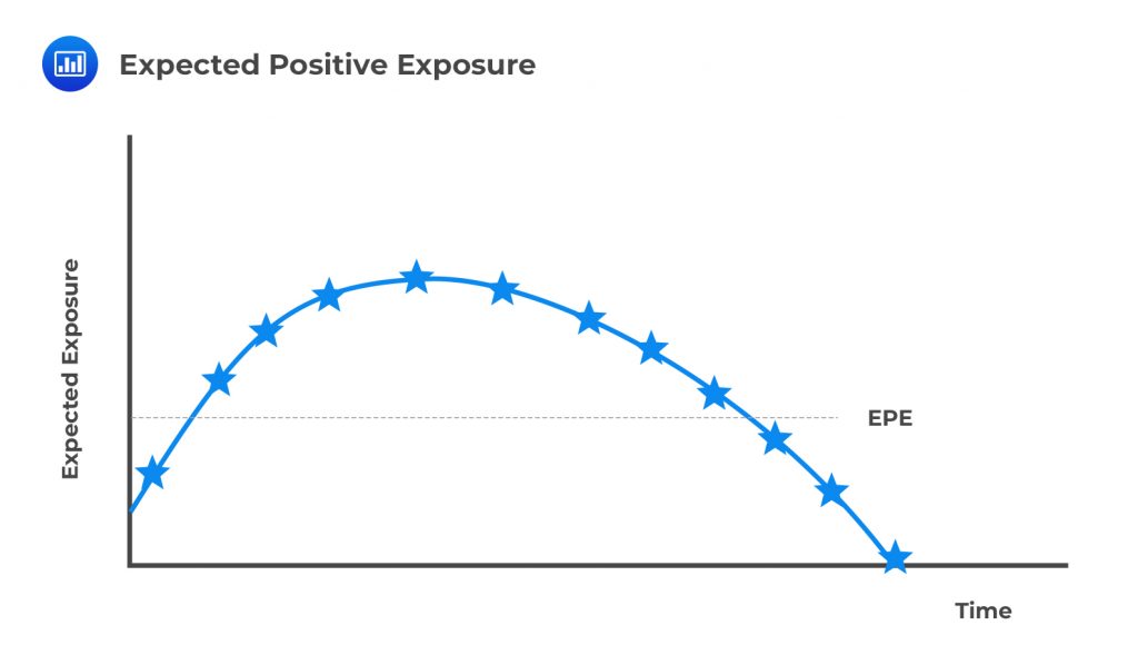
We can adopt a very similar model to calculate stress loss in derivative transactions. This time, however, we assume that the probability of default and loss-given default of the counterparty is the same. The expected positive exposure is, nonetheless, stochastic and depends on the levels of market variables. Instead of using exposure at default (EAD), we use the expected positive exposures (EPE), which is the weighted average over time of expected exposure, multiplied by an alpha factor α. We can see that the following aspects will all cause a decrease in the value of alpha:
$$ \begin{array}{l|c} \textbf{ } & \textbf{Alpha} \\ \hline \text{Infinitely large ideal portfolio} & \text{1.0} \\ \hline \text{Canabarro et al. (2003)} & \text{1.09} \\ \hline \text{Wilde (2005)} & \text{1.21} \\ \hline \text{ISDA (2003)} & \text{1.07-1.10} \\ \hline \text{Regulatory prescribed value} & \text{1.4} \\ \hline \text{Supervisory floor (if using own estimation)} & \text{1.2} \\ \hline \text{Possible values for concentrated portfolios} & \text{2.5 or more} \\ \end{array} $$
The expected loss and the stressed expected loss can then be measured as follows:
$$ \text{EL}=\sum _{ \text{i}=1 }^{ \text{N} }{ { \text{PD} }_{ \text{i} } } \times \alpha \times { \text{EPE} }_{ \text{i} }\times { \text{LGD} }_{ \text{i} } $$
$$ \text{EL}_{ \text{s} }=\sum _{ \text{i}=1 }^{ \text{N} }{ { \text{PD} }_{ \text{i} }^{ \text{s}} } \times \alpha \times { \text{EPE} }_{ \text{i} }^{ \text{s} }\times { \text{LGD} }_{ \text{i} } $$
An institution can calculate stress losses on the derivatives portfolio the same way it does on the loan portfolio. Remember that stressed values of the probability of default can be obtained by stressing the probability of default itself or tweaking the variables that affect it. These variables include things such as assets and liabilities on the balance sheet, macroeconomic indicators, as well as values of financial instruments. It is also possible to get a comprehensive stress report by cumulatively adding the stress losses on the loan portfolio and the stress losses on its derivatives portfolio.
When carrying out stress tests on derivative transactions, there’s a wide range of variables to stress. The value attached to the EPE, which measures the exposure, depends on variables such as equity prices and swap rates. Each of these variables can be tweaked to see how they affect the expected loss. It is important to note that a stress event can, in the aggregate, increase or decrease the expected losses. The impact will depend on many factors, including any bias in the composition of a bank’s portfolio and margining among counterparties. However, it must also be noted that stresses on the probability of default affect all positions in the same direction.
In the same vein, financial institutions shock a series of market variables instantaneously. The initial value of a derivative is shocked prior to the simulation process to calculate the EPE. How this shock affects the EPE will depend, in part, on the degree of collateralization and the moneyness of the portfolio. Although a series of shocks could also be performed over a period of time, most financial institutions tend to perform shocks to current exposure only.
It is also possible to look at the joint stresses of credit quality and market variables. In theory, this sounds like a straightforward exercise. Note, however, that in practice, coming up with a model that estimates the relationship between macroeconomic variables or balance-sheet variables and changes in market variables can be daunting.
Equally daunting is the attempt to establish a link between PD and exposure or rather, wrong-way risk. At present, there are many methods of capturing wrong-way risk but most of them are ad hoc. The best way an institution can identify wrong-way risk in the credit framework would involve stressing the current exposure, identifying those counterparties that are most exposed to the stress, and then carefully considering whether the counterparty is also subject to wrong-way risk or not.
When stress-testing CCR in a market risk context, financial institutions look at the market value of the counterparty credit risk and evaluate losses that could be realized if various market variables, including the credit spread of the counterparty, change.
In many cases, a financial institution will consider its unilateral CVA for stress testing. That means the institution explores the market scenarios that could lead to counterparty default. But as we have seen previously, all derivative transactions tend to have bilateral counterparty risk. It is, therefore, important for the financial institution to take its own default to the counterparty into account. It is equally important to consider the bilateral CVA, not just the unilateral CVA, during stress testing.
The following simplified example gives the CVA to a counterparty, without taking into account wrong-way risk:
$$ { { \text{CVA} } }_{ \text{n} }={ { { { \text{LGD} } } }_{\text n }^{ * } }\times \sum _{ {\text j }={\text i } }^{ {\text T } }{ { \text{EE} }_{\text n }^{ * } } \left( { {\text t } }_{ {\text j } } \right) \times { \text q }_{\text n }^{ * }\left( { {\text t } }_{ {\text j }-1 },{ {\text t } }_{ {\text j } } \right) $$
Where:
\({ { { \text{EE} }_{ \text{n} }^{ \text{*}} } } \left( { \text{t} }_{ \text{j} } \right)\) is the discounted expected exposure during the jth time period computed under a risk-neutral measure for counterparty n;
\({ { \text{q} }_{ \text{n} }^{ \text{*}} }\left( { \text{t} }_{ \text{j}-1 },{ \text{t} }_{ \text{j} } \right) \) is the risk-neutral marginal default probability for counterparty n between period \({ \text{t} }_{ \text{j}-1 }\) and \({ \text{t} }_{ \text{j} }\) with T being the final maturity; and
\( {{{ \text{LGD} }_{ \text{n} }^{ * }} }\) is the risk-neutral loss-given default for counterparty n.
When aggregating across N counterparties in a portfolio, the CVA formula becomes:
$$ { \text{CVA} }=\sum _{ \text{n}=1 }^{ \text{N} }{ { { \text{LGD} }_{ \text{n} }^{ * }} } \times \sum _{ \text{j}=\text{i} }^{ \text{T} }{ { { \text{EE} }_{ \text{n} }^{ \text{*} }} } \left( { \text{t} }_{ \text{j} } \right) \times { { \text{q} }_{ \text{n} }^{ \text{*}} }\left( { \text{t} }_{ \text{j}-1 },{ \text{t} }_{ \text{j} } \right) $$
It is important to bear in mind that all of the key components in the above formulas are dependent on market variables. In particular,
\({ { \text{q} }_{ \text{n} }^{ \text{*}} }\left( { \text{t} }_{ \text{j}-1 },{ \text{t} }_{ \text{j} } \right) \) is derived from the counterparty’s credit spread;
\( {{{ \text{LGD} }_{ \text{n} }^{ * }} }\) is set by convention or from market spreads, and;
\({ { { \text{EE} }_{ \text{n} }^{ \text{*}} } } \left( { \text{t} }_{ \text{j} } \right)\) is dependent on the values of the derivative contract with the counterparty.
The stressed CVA is calculated by applying instantaneous shocks to some of these variables. These stresses affect the risk-neutral discounted expected exposure, \({ { { \text{EE} }_{ \text{n} }^{ \text{*}} } } \left( { \text{t} }_{ \text{j} } \right)\) as well as the risk-neutral marginal default probability, \({ { \text{q} }_{ \text{n} }^{ \text{*} }}\left( { \text{t} }_{ \text{j}-1 },{ \text{t} }_{ \text{j} } \right) \)
The stressed CVA can be calculated as:
$$ { \text{CVA} }^{ \text{s} }=\sum _{ \text{n}=1 }^{ \text{N} }{ { { \text{LGD} }_{ \text{n} }^{ * }} } \times \sum _{ \text{j}=\text{i} }^{ \text{T} }{ { { \text{EE} }_{ \text{n} }^{ \text{s}} } } \left( { \text{t} }_{ \text{j} } \right) \times { { \text{q} }_{ \text{n} }^{ \text{s} }}\left( { \text{t} }_{ \text{j}-1 },{ \text{t} }_{ \text{j} } \right) $$
Stress loss, as illustrated earlier, is the difference between the stressed CVA and the current CVA.
$$ { \text{CVA} }^{ \text{s} }-\text{current CVA}=\text{Stress loss} $$
We can draw parallels between stress testing CCR in a credit risk framework and stress testing in a market risk framework. What particularly stands out is that in both cases, expected losses are the product of the loss-given default, exposure, and probability of default. However, these values will be quite different, depending on the view of CCR as market risk or credit risk. There are several reasons behind the differences, but the main ones are:
Why is it so important to use a market-based model for the probability of default?
It makes it possible to incorporate a correlation between PD and exposure (wrong-way risk). This correlation has the potential to significantly influence the CVA. However, this also means that institutions have an obligation to closely monitor the correlation value because an incorrect value can have a serious effect on the simulated profit and loss values.
A one-year CDS has the following characteristics:
The risk-free rate is 5%.
Question 1: What is the CVA?
$$ \text{Average default intensity (hazard rate, λ)} =\frac{s}{1-R}=\frac{0.02}{1-40/%} = 0.0333 $$
$$ \text{Marginal default probability} = λe^{-λt}=0.0333e^{-0.0333×1}=3.22\% $$
$$\begin{align*} { { \text{CVA} } }_{ \text{n} }&={ { { { \text{LGD} } } }_{\text n }^{ * } }\times \sum _{ {\text j }={\text i } }^{ {\text T } }{ { \text{EE} }_{\text n }^{ * } } \left( { {\text t } }_{ {\text j } } \right) \times { \text q }_{\text n }^{ * }\left( { {\text t } }_{ {\text j }-1 },{ {\text t } }_{ {\text j } } \right) \\ &= (1-40\%)×30,000,000e^{-1×5\%}×3.22\%=551,332 \end{align*}$$
Note: To see how to compute the marginal default probability, go back to the chapter on Spread Risk and Default Intensity Models. There is a high likelihood you will be getting a quick on this in your FRM Part 2 exam.
Question 2:If we were to shock the expected exposure and the probability of default by increasing them both by 50%, what would be our stress loss?
$$\begin{align*} { \text{CVA} }^{ \text{s} }&= { { { \text{LGD} }_{ \text{n} }^{ * }} } \times{ { { \text{EE} }_{ \text{n} }^{ \text{s}} } } \left( { \text{t} }_{ \text{j} } \right) \times { { \text{q} }_{ \text{n} }^{ \text{s} }}\left( { \text{t} }_{ \text{j}-1 },{ \text{t} }_{ \text{j} } \right) \\ &=(1-40\%)×(30,000,000e^{-1×5\%}×1.5)×(3.22\%×1.5)=1,240,498\end{align*} $$
$$\begin{align*} \text{Stress loss} &= \text{Stress BCVA} – \text{Current BCVA}\\& = 1,240,498-551,332=689,166\end{align*} $$
As mentioned previously, it is important that a financial institution considers not just A counterparty’s risk of default but also its own default to the counterparty. This will ensure that the institution gets a more accurate view of the impact of various scenarios on CVA profit and loss. The formula for DVA is pretty similar to the one for CVA, but there are two notable changes:
The bilateral CVA formula is given as:
$$ \begin{align*} \text{BCVA} & =+\sum _{ \text{n}=1 }^{ \text{N} }{ { { \text{LGD} }_{ \text{n} }^{ * }} } \times \sum _{ \text{j}=i }^{ \text{T} }{ { { \text{EE} }_{ \text{n} }^{ * }} } \left( { \text{t} }_{ \text{j} } \right) \times { { \text{q} }_{ \text{n} }^{ * }} \left( { \text{t} }_{ \text{j}-1 },{ \text{t} }_{ \text{j} } \right) \times { { \text{S} }_{ 1 }^{ * }} \left( { \text{t} }_{ \text{j}-1 } \right) \\ & -\sum _{ \text{n}=1 }^{ \text{N} }{ { { \text{LGD} }_{ 1 }^{ * }} } \times \sum _{ \text{j}=i }^{ \text{T} }{ { \text{N}{ \text{EE} }_{ \text{n} }^{ * }} } \left( { \text{t} }_{ \text{j} } \right) \times { { \text{q} }_{ 1 }^{ * }} \left( { \text{t} }_{ \text{j}-1 },{ \text{t} }_{ \text{j} } \right) \times { { \text{S} }_{ \text{j} }^{ * }} \left( { \text{t} }_{ \text{j}-1 } \right) \end{align*} $$
We make two important observations:
The first one is that in this formulation, the survival probabilities also depend on CDS spreads and the losses depend on the firm’s own credit spread. This may yield counterintuitive results. For instance, a loss may occur because of an improvement in the firm’s own credit quality.
The second one is that when looking at stress tests from a bilateral perspective, it is important that the financial institution considers how its own credit spread is correlated with its counterparties’ credit spread.
Finally, stress losses can be calculated in a similar way as for CVA losses:
$$ \text{Stress loss} = \text{Stress BCVA} – \text{Current BCVA} $$
The BCVA approach to stress testing is important because it allows CCR to be treated as a market risk. This means that CCR can be incorporated into market risk stress testing in a consistent manner. BCVA stress results could then be added to the institution’s stress tests from market risk.
Stress testing CCR comes with the following pitfalls:
Practice Question
Financial institutions use stress tests of CCR as a credit risk which allows them to advance beyond simple stresses of current exposure. These tests permit the accumulation of losses due to loan portfolios and also take the credit quality of the counterparty into account . These are considered important developments that allow financial institutions to better manage their portfolio of derivatives. When stress testing CCR in the context of market risk, we are usually concerned with:
A.The market value of the counterparty’s credit risk and the losses that could result due to changes in market variables, including the credit spread of the counterparty.
B.The market value of the counterparty’s collaterals and the losses that could be occasioned by changes in market variables, including the credit spread of the counterparty.
C.The size of individual cash flows and the losses that could result due to changes in market variables.
D.The market value of the counterparty’s collaterals and the losses that could result due to changes in macroeconomic variables, including the fluctuations in the market variables.
The correct answer is A.
When stress testing CCR in a market risk context, we are usually concerned with the market value of the counterparty’s credit risk and the losses that could result due to changes in market variables, including the credit spread of the counterparty.
Offered by AnalystPrep


Get Ahead on Your Study Prep This Cyber Monday! Save 35% on all CFA® and FRM® Unlimited Packages. Use code CYBERMONDAY at checkout. Offer ends Dec 1st.