Non-Parametric Approaches

p>

After completing this reading, you should be able to:

• Apply the bootstrap historical simulation approach to estimate coherent risk measures.
• Describe historical simulation using non-parametric density estimation.
• Compare and contrast the age-weighted, the volatility-weighted, the correlation-weighted, and the filtered historical simulation approaches.
• Identify the advantages and disadvantages of nonparametric estimation methods.

The Bootstrap Historical Simulation Approach to Estimating Coherent Risk Measures

Bootstrapping presents a simple but powerful improvement over basic Historical Simulation. It is employed in the estimation of VaR and ES. It assumes that the distribution of returns will remain the same in the past and in the future, justifying the use of historical returns to forecast the VaR.

A bootstrap procedure involves resampling from our existing data set with replacement. A sample is drawn from the data set, its VaR recorded, and the data “returned.” This procedure is repeated over and over. The final VaR estimate from the full data set is taken to be the \(\textbf{average}\) of all sample VaRs. In fact, bootstrapped VaR estimates are often more accurate than ‘raw’ sample estimates.

There are three key points to note regarding a basic bootstrap exercise:

1. We start with a given original sample of size n. We then draw a new random sample of the same size from this original sample, “returning” each chosen observation to the sampling pool after it has been drawn.

2. Sampling with replacement implies that some observations get chosen more than once while others don’t get chosen at all. In other words, a new sample, known as a resample, may contain multiple instances of a given observation or leave out the observation completely, making the resample different from both the original sample and other resamples. From each resample, therefore, we get a different estimate of our parameter of interest.

3. The resampling process is repeated many times over, resulting in a set of resampled parameter estimates. In the end, the average of all the resample parameter estimates gives us the final bootstrap estimate of the parameter. The bootstrapped parameter estimates can also be used to estimate a confidence interval for our parameter of interest.

Equally important is the possibility of extending the key tenets of bootstraps to the estimation of the expected shortfall. Each drawn sample will have its own ES. First, the tail region is sliced up into n slices and the VaR for each of the resulting n – 1 quantiles is determined. The final VaR estimate is taken to be the average of all the tail VaRs.We then estimate the ESas the average of losses in excess of the final VaR.

As in the case of the VaR, the best estimate of the expected shortfall given the original data set is the average of all of the sample expected shortfalls.

In general, this bootstrapping technique consistently provides more precise estimates of coherent risk measures than historical simulation of raw data alone.

Bootstrapped Confidence Intervals

For a start, we know that thanks to the central limit theorem, the distribution of \(\widehat { \theta } \)often approaches normality as the number of samples gets large. In these circumstances, it would be reasonable to estimate a confidence interval for θ assuming \(\widehat { \theta }\) is approximately normal.

Given that \(\widehat { \theta }\) is our estimate of θ and \(\widehat { \sigma }\) is the estimate of the standard error of \(\widehat { \theta } \), the confidence interval at 95% is: $$ [\widehat { \theta }-1.96\widehat { \sigma },\widehat { \theta } +1.96 \sigma ̂] $$

It is also possible to work out confidence intervals using percentiles of the sample distribution. The upper and lower bounds of the confidence interval are given the percentile points (or quantiles)of the sample distribution of parameter estimates.

Historical Simulation Using Non-parametric Density Estimation

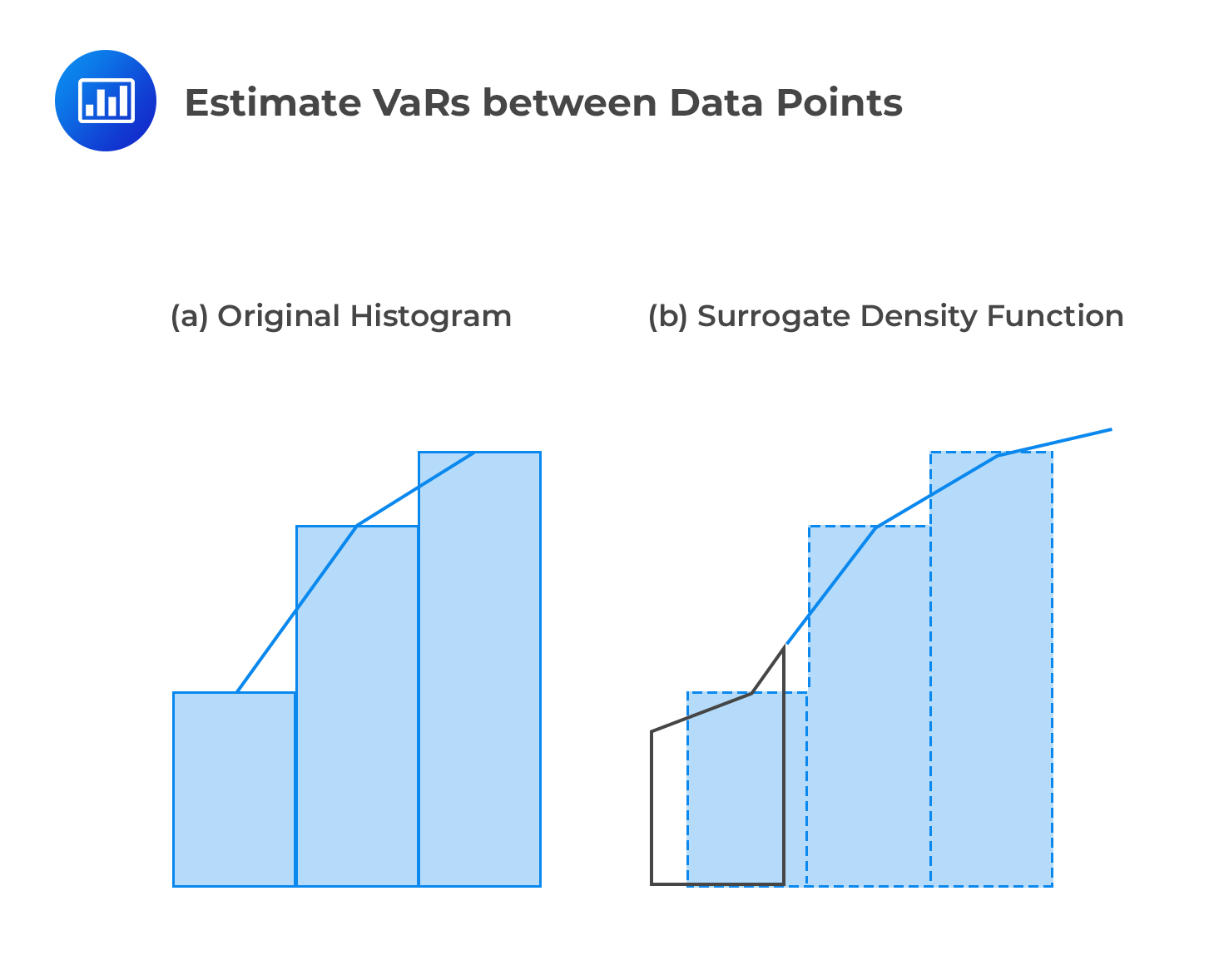
A huge selling point about the traditional historical approach has much to do with its simplicity. However, there’s one major drawback: due to the discrete nature of data, it is impossible to estimate VaRs between data points. For example, if there are 100 historical observations, it would be easy to estimate the VaR at 95% or even 99%. But what about the VaR at, say, 96.5%? It would be impossible to incorporate a level of confidence of 96.5%. The point here is that with n observations, the historical simulation method only allows for n different confidence levels. Luckily, Non-parametric density estimation offers a potential solution to this problem.

So what happens? We treat our data as drawings that are free from the “shackles” of some specified distribution. The idea is to make the data “speak for itself” without making any strong assumptions about its distribution. To enable us estimate VaRs and ESs for any confidence levels, we simply draw straight lines connecting the mid-points at the top of each histogram bar (in the original data set’s distribution) and treat the area under the lines as if it were a pdf. By so doing, don’t we lose part of the data? No: by connecting the midpoints, the lower bar “receives” some area from the upper bar, which “loses” or cedes an equal amount of area. In the end, no area is lost, only displacement occurs. We still end up with a probability distribution function. The shaded area in the figure below represents a possible confidence interval that can be utilized regardless of the size of the data set.

Weighted Historical Simulation Approaches

Remember that under the historical method of estimating VaR, all of the past n observations are weighted equally. In addition, each observation has a weight of 1/n. In other words, our HS P/L series is constructed in a way that gives any observation n periods old or less the \(\textbf {same}\) weight in our VaR, and \(\textbf {no}\) weight (i.e., a zero weight) to all observations that come after that. Even though its construction is simple, this weighting scheme has several flaws.

To begin with, it seems hard to justify giving each observation the same weight without taking its age, market volatility at the time it was observed, or the value it takes into account. For instance, it’s an open secret that gas prices are more volatile in winter than in summer. So, if the sample period cuts across the two seasons of the year, the resulting VaR estimate will not reflect the true risk facing the firm under review. As a matter of fact, equal weights will tend to underestimate true risks in winter and overestimate them in summer.

Moreover, equal weights make the resulting risk estimates unresponsive to major events. For instance, we all know that risk increases significantly following a major destabilizing event such as a stock market crash or the start of a trade war involving one or more economies (the US and China would be perfect examples). Unless a very high level of confidence is used, HS VaR estimates won’t capture the increased risk following such events. The increase in risk would only reflect in subsequent dates if the market slide continues.

Aside from all the flaws cited in the foregoing paragraphs, equal weights suggest that each observation in the sample period is equally likely and independent of all the others. That is untrue because, in practice, periods of high or low volatility tend to be clustered together.

An equally noteworthy flaw is that an unusually high observation will tend to have a major influence on the VaR until n days have passed and the observation has fallen out of the sample period, at which point the VaR will fall again.

Finally, it would be difficult to justify a sudden shift of weight from 1/n on date n to zero on date n+1. In other words, it would be hard to explain why the observation on date n is important while the one on date n+1 is not.

This learning outcome looks at four improvements to the traditional historical simulation method.

Age-weighted Historical Simulation (Hybrid HS)

Instead of equal weights, we could come up with a weighting structure that discounts the older observations in favor of newer ones.

Let the ratio of consecutive weights be constant at lambda (\(\lambda\)). If w(1) is the probability weight given to an observation that’s 1 day old, then w(2), the probability given to a 2-day old observation could be \(\lambda\)w(1); w(3), the probability weight given to a 3-day  old observation could be \(\lambda^2\) w(1); w(4) could be \(\lambda^3\) w(1,), w(5) could be \(\lambda^4\) w(1), and so on. In such a case, lambda would be a term between 0 and 1 and would reflect the exponential rate of decay in the weight as time goes. A\(\lambda\) close to 1 signifies a slow rate of decay, while a \(\lambda\) far away from 1 signifies a high rate of decay.

Under age-weighted historical simulation, therefore, the weight given to an observation i days old is given by:

$$ w(i)=\cfrac {\lambda^{i-1} (1-\lambda)}{(1-\lambda^n ) } $$

w(1) is set such that the sum of the weights is 1.

Example

$$ \bf{\lambda = 0.96;} \bf{{\text n}=100} $$

$$ \textbf{Initial date} $$

$$ \textbf{listing only the worst 6 returns} $$

$$ \begin{array}{c|c|cc|cc} {} & {} & \textbf{Simple} & \textbf{HS} & \textbf{Hybrid} & \textbf{(Exp)} \\ \hline \textbf{Return} & \textbf{periods ago(i)} & \textbf{Weight} & \textbf{Cumul.} & \textbf{Weight} & \textbf{Cumul.} \\ \hline {-3.50\%} & {6} & {1.00\%} & {1.00\%} & {3.32\%} & {3.32\%} \\ \hline {-3.20\%} & {4} & {1.00\%} & {2.00\%} & {3.60\%} & {6.92\%} \\ \hline {-2.90\%} & {55} & {1.00\%} & {3.00\%} & {0.45\%} & {7.37\%} \\ \hline {-2.70\%} & {35} & {1.00\%} & {4.00\%} & {1.02\%} & {8.39\%} \\ \hline {-2.60\%} & {8} & {1.00\%} & {5.00\%} & {3.06\%} & {11.45\%} \\ \hline {-2.40\%} & {24} & {1.00\%} & {6.00\%} & {1.60\%} & {13.05\%} \end{array} $$

$$ \bf{\lambda = 0.96; {\text n}=100} $$

$$ \textbf{20 days later} $$

$$ \textbf{Note: Only the 6th worst return is recent. The others are same} $$

$$ \begin{array}{c|c|cc|cc} {} & {} & \textbf{Simple} & \textbf{HS} & \textbf{Hybrid} & \textbf{(Exp)} \\ \hline \textbf{Return} & \textbf{periods ago(i)} & \textbf{Weight} & \textbf{Cumul.} & \textbf{Weight} & \textbf{Cumul.} \\ \hline {-3.50\%} & {26} & {1.00\%} & {1.00\%} & {1.47\%} & {1.47\%} \\ \hline {-3.200\%} & {24} & {1.00\%} & {2.00\%} & {1.59\%} & {3.06\%} \\ \hline {-2.90\%} & {75} & {1.00\%} & {3.00\%} & {0.20\%} & {3.26\%} \\ \hline {-2.70\%} & {55} & {1.00\%} & {4.00\%} & {0.45\%} & {3.71\%} \\ \hline {-2.60\%} & {28} & {1.00\%} & {5.00\%} & {1.35\%} & {5.06\%} \\ \hline \bf{-2.50\%} & \bf{14} & \bf{1.00\%} & \bf{6.00\%} & \bf{2.39\%} & \bf{7.45\%} \end{array} $$

$$ w(i)=\cfrac {\lambda^{i-1} (1-\lambda)}{(1-\lambda^n ) } \quad \quad \text{e.g. }w(6)=\cfrac {0.96^{6-1} (1-0.96)}{(1-0.96^{100} ) }=3.32\% $$

Advantages of the age-weighted HS method include:

• It generalizes standard historical simulation (HS) because “we can regard traditional HS as a special case with zero decay, where \(\lambda\) is essentially equal to 1.
• Choosing lambda appropriately will make VaR/ES estimates more responsive to large loss observations. A suitable choice of lambda will award a large loss event a higher weight than traditional HS, making the resulting next day VaR higher than it would otherwise have been.
• It helps to reduce distortions caused by events that are unlikely to recur and helps to reduce ghost effects. An unusually large loss will have its weight gradually reduced as time goes by until it is “kicked out” of the historical sample size.
• Age-weighting can be modified in a way that renders VaR and ES more efficient.

Volatility-weighted Historical Simulation

Instead of weighting individual observations by proximity to the current date, we can also weight data by relative volatility. This idea was originally put forth by Hull and White to incorporate changing volatility in risk estimation. The underlying argument is that if volatility has been on the rise in the recent past, then using historical data will \(\textbf{underestimate}\) the current risk level. Similarly, if current volatility has significantly reduced, then using historical data will \(\textbf{overstate}\) the current risk level.

If \(\text r_{\text t}\),i, is the historical return in asset i on day t in our historical sample, \(\sigma_{t,i}\), the historical GARCH (or EWMA) forecast of the volatility of the return on asset i for day t, and \(\sigma_{T,i}\), the most recent forecast of the volatility of asset i, then the volatility-adjusted return is:

$$ \text r_{\text t,\text i}^*=\cfrac {\sigma_{\text T,\text i}}{\sigma_{\text t,\text i}} \text r_{\text t,\text i} $$

Actual returns in any period t will therefore increase (or decrease), depending on whether the current forecast of volatility is greater (or less) than the estimated volatility for period t.

Advantages of the volatility-weighted approach relative to equal-weighted or age-weighted approaches include:

• The approach explicitly incorporates volatility into the estimation procedure. The equal-weighted HS completely ignores volatility changes. Although the age-weighted approach recognizes volatility, its treatment is rather arbitrary and restrictive.
• The method produces near-term VaR estimates that are likely to be more sensitive to current market conditions.
• Volatility-adjusted returns accommodate VaR and ES estimates that can exceed the maximum loss in our historical data set. Under traditional HS, VaR or ES cannot be bigger than the losses in our historical data set.
• Empirical evidence indicates that this approach produces VaR estimates that are superior to the VaR estimates under the age-weighted approach.

Correlation-weighted Historical Simulation

Historical returns can also be adjusted to reflect changes between historical and current correlations. In other words, this method incorporates updated correlations between asset pairs. In essence, the historical correlation (or equivalently variance-covariance) matrix is adjusted to the new information environment by “multiplying” the historic returns by the revised correlation matrix to yield updated correlation-adjusted returns.

Suppose there are \(m\) positions in the portfolio. Suppose further that historical returns \(R\) for a specific time period \(t\) have already been adjusted for volatility. This \(1\times m\) vector of these returns reflects the\(m\times m\) variance-covariance matrix which is denoted as Σ.

The variance-covariance matrix Σ can be decomposed into the product \(\sigma{C}\sigma^{T}\) where \(\sigma\) is \(m\times m\) diagonal matrix of volatilities with the i^th element being the i^th volatility \(\sigma_i\)​, and off-diagonal elements being zero. \(\sigma^T\)​, is the transpose of \(\sigma_i\). \(C\) is the \(m\times m\) matrix of historical correlations.

Thus, \(R\) reflects a historical correlation matrix \(C\) and the goal is to adjust \(R\) to \(\bar{R}\) so that they reflect the current matrix, \(\bar{C}\). Assuming both correlation matrices are positive definite, they can be decomposed using Cholesky decomposition.

Each correlation matrix has an \(m\times m\) ‘matrix square root,’ denoted as \(A\) and \(\bar{A}\), respectively. Now, we can represent \(R\) and \(\bar{R}\) as matrix products of the relevant Cholesky matrices and an uncorrelated noise process \(e\):

$$R=Ae … … …\text{eqn. i}$$

$$\bar{R} = \bar{A}e … … …\text{eqn. ii}$$

From eqn. i above,

$$e = A^{-1}R$$

Substituting this result in eqn. ii above, we obtain the correlation-adjusted series \(\bar{R}\) that represents the desired correlations:

$$\bar{R}= \bar{A}*A^{-1}R$$

The adjusted returns, \(\bar{R}\) will reflect the currently prevailing correlation matrix \(\bar{C}\) and, more generally, the currently prevailing covariance matrix \(\bar{Σ}\).

Filtered Historical Simulation

The filtered historical simulation is undoubtedly the most comprehensive, and hence most complicated, of the non-parametric estimators. The method aims to combine the benefits of historical simulation with the power/flexibility of conditional volatility models(such as GARCH or asymmetric GARCH).

Steps involved:

1. A conditional volatility model (e.g., GARCH) is fitted to our portfolio-return data.
2. Actual returns are translated into standardized returns.
3. The conditional volatility model is used to forecast volatility for each of the days in a sample period.
4. These volatility forecasts are then divided into the realized returns to produce a set of standardized returns that are iid (independent and equally distributed).
5. A bootstrapping exercise is performed assuming a 1-day VaR holding period.
6. The VaR is computed

Advantages and Disadvantages of Non-parametric Methods

Advantages

1. They are instinctive and conceptually simple.
2. They can accommodate fat tails, skewness, and other features that are, otherwise, abnormal to parametric approaches.
3. They can accommodate any type of position including derivative positions.
4. HS works quite well empirically.
5. In varying degrees, they are quite easy to implement on a spreadsheet.
6. They are free of operational problems.
7. They use readily available data.
8. Results provided are easily reported and communicated to seniors.
9. Confidence intervals for non-parametric VaR and ES are easily produced.
10. When combined with add-ons, they are capable of refinement and potential improvement.

Disadvantages

1. For unusually quiet data periods, VaR and ES estimates are too low for actual risks faced.
2. For unusually volatile data periods, the estimates for VaR or ES produced are too high.
3. Difficulty in handling shifts during sample periods.
4. An extreme loss in the data set dominates non-parametric risk estimates.
5. Subject to the phenomenon of ghost effect or shadow effects.
6. They are constrained by the largest loss in historical data.

Practice Question

Assume that Mrs. Barnwell, a risk manager, has a portfolio with only 2 positions. The two positions have a historical correlation of 0.5 between them. She wishes to adjust her historical returns \(R\) to reflect a current correlation of 0.8. Which of the following best reflects the 0.8 current correlation?

1. \(\left( \begin{matrix} 1 & 0.3464 \\ 0 & 0.6928 \end{matrix} \right) R\).
2. \(\begin{pmatrix} 0 & 0.3464 \\ 1 & 0.6928 \end{pmatrix}R\).
3. \(\begin{pmatrix} 1 & 0 \\ 0.3464 & 0.6928 \end{pmatrix}R\).
4. \(0.96R\)

Correct answer is C.

Note that if \({ a }_{ i,j }\) is the \(i\), \(jth\) element of the 2 x 2 matrix \(A\), then by applying Choleski decomposition, \({ a }_{ 11 }=1\), \({ a }_{ 12 }=0\), \({ a }_{ 21 }=\rho ,{ a }_{ 22 }=\sqrt { 1-{ \rho }^{ 2 } } \). From Our data, \({ \rho }\) = 0.5, Matrix \(\overline { A } \) is similar but has a \({ \rho } = 0.8\).

Therefore:

$$ { A }^{ -1 }=\frac { 1 }{ { a }_{ 11 }{ a }_{ 22 }-{ a }_{ 12 }{ a }_{ 21 } } \begin{pmatrix} { a }_{ 22 } & { -a }_{ 12 } \\ { -a }_{ 21 } & { a }_{ 11 } \end{pmatrix} $$

Substituting

$$ \hat { R } =\overline { A } { A }^{ -1 }R $$

We get

$$ \begin{pmatrix} 1 & 0 \\ 0.8 & \sqrt { 1-{ 0.8 }^{ 2 } } \end{pmatrix}\frac { 1 }{ \sqrt { 1-{ 0.5 }^{ 2 } } } \begin{pmatrix} \sqrt { 1-{ 0.5 }^{ 2 } } & 0 \\ -0.5 & 1 \end{pmatrix}R $$

$$ =\begin{pmatrix} 1 & 0 \\ 0.3464 & 0.6925 \end{pmatrix}R $$