


Messages from the Academic Literature ...
After completing this reading, you should be able to: Explain the following lessons... Read More

After completing this reading, you should be able to:
Financial correlation risk is the risk of financial loss due to adverse movements in the correlation between two or more (financial) variables. It is the risk that the correlation between two or more variables changes unfavorably. An increase in asset return correlations increases the risk of financial loss.
The issue of correlation risk came to the fore during the 2007/2009 financial crisis where a dramatic increase in correlation was witnessed across the financial industry. For example, an increase in default correlation between bond issuers and insurers was observed, which represents a wrong-way risk.
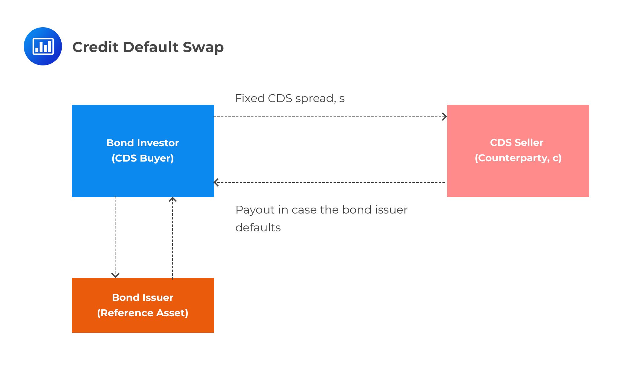 A CDS works to transfer credit risk from an investor to a counterparty. It’s more like an insurance policy. Let’s look at a typical scenario.
Assume that an investor has invested some $100 million in bonds issued by Italy but is worried that there might be a default event in light of a persistent trade war. To hedge default risk, the investor buys a CDS from a Spanish bank, La Mada. The CDS shields the investor from defaulted-related losses; in case Italy defaults, the counterparty, La Mada, will pay the originally invested $100.0 million to the investor (assuming the recovery rate is zero). The key thing to note here is that the value of the CDS, the fixed CDS spread s, is determined by the default probability of the reference asset – Italy. The “spread” of a CDS is the annual amount, expressed as a percentage of the notional amount, that an investor must pay the counterparty (protection seller) over the length of the contract.
The value of the CDS is also determined by the joint default correlation of La Mada and Italy. If the correlation between Italy and La Mada increases, the present value of the CDS for the investor will decrease in which case, they will suffer an unrealized (paper) loss. Therefore, the investor is exposed to default correlation risk between the reference asset (Italy) and the counterparty (La Mada). In the worst-case scenario where the reference entity and La Mada jointly default, the investor stands to lose all of their investment.
The fact that both Italy and Spain are in Europe (and the European Union) implies that there would most likely be a positive default correlation between them. This implies that the investor has a wrong-way risk. The higher the correlation risk, the lower the CDS spread,s. That’s because an increase in correlation means a higher probability of the reference asset and the counterparty defaulting together (the investor would want to pay a lower premium if the probability of losing his investment increases).
Other examples of financial correlation risk include:
Negative correlation in the context of a CDS implies that there’s a low probability of joint default. In the above example, a high negative correlation implies that either Italy or La Mada will default, but not both. If Italy defaults, the $100 million is recovered from La Mada. If La Mada defaults, the investor loses the value of the CDS spread and they will have to go back into the market to repurchase a CDS spread to hedge the position. The cost will be higher if the credit quality of Italy has decreased since the inception of the original CDS.
Sometimes, the dependencies between the CDS spread, s, and correlation risk may be nonmonotonous. What does that mean? The CDS spread may show some inconsistency by increasing and, sometimes, decreasing if correlation risk increases.
The capital asset pricing model (CAPM) tells us that an increase in diversification increases the return/risk ratio. There exists an inverse relationship between correlation and diversification; High diversification is related to low correlation. The lower the correlation of the assets in a portfolio, the higher the return/risk ratio.
To further explain this, consider a return on asset X at time t as \(x_t\), and let \(y_t\) be the return of asset Y at time t. A return is calculated as a percentage change, \((S_t – S_{t-1})/S_{t-1}\), where S is a price or a rate.
The average returns of asset X and Y are \(\mu_X\) and \(\mu_Y\), respectively. Assigning the weight \(W_x\) to asset X and \(W_Y\) to asset Y,
where \(W_x+ W_Y = 1\)
Where n is the number of observed points in time.
We can calculate the standard deviation of returns of Y in a similar manner:
$$ \sigma_Y=\sqrt { \cfrac {1}{n-1} \sum_{t=1}^n(y_t-\mu_Y)^2 } $$
Returns on both assets tend to be on the same side (above or below) their expected values at the same time (an average positive relationship between returns).
When the return on one asset is above its expected value, the return on the other asset tends to be below its expected value (an average inverse relationship between returns).
Returns on the assets are unrelated.
Covariance is not easy to interpret since it takes values between \(−\infty\) and \(+\infty\). It is more convenient to standardize covariance in the form of the Pearson correlation coefficient \(\rho_{XY}\).
There’s a strong positive linear relationship (up to 1, which indicates a perfect linear relationship).
There’s a strong negative (inverse) linear relationship (down to −1, which indicates a perfect inverse linear relationship).
There’s NO linear relationship.
In finance, the standard deviation is interpreted as risk. The higher the standard deviation, the higher the risk of an asset or a portfolio.
The following table gives the returns of two assets, X and Y, over a six-year period. The weight of X is equal to that of Y.
$$ \begin{array}{l|c|c|c|c}\textbf{Year} & \textbf{Asset X} & \textbf{Asset Y} & \textbf{Return of X} & \textbf{Return of Y} \\ \hline {2008} & {100} & {200} & {} & {} \\ \hline {2009} & {120} & {230} & {20.00\%} & {15.00\%} \\ \hline {2010} & {108} & {460} & {-10.00\%} & {100.00\%} \\ \hline {2011} & {190} & {410} & {75.93\%} & {-10.87\%} \\ \hline {2012} & {160} & {480} & {-15.79\%} & {17.07\%} \\ \hline {2013} & {280} & {380} & {75.00\%} & {-20.83\%} \\ \hline {} & {} & \text{Average} & {29.03\%} & {20.07\%}\end{array} $$
Tasks:
Interpretation: X and Y show an average inverse relationship. When the return on one asset is above its expected value, the return on the other asset tends to be below its expected value. In fact, a look at the table confirms that this is the case in the years 2010, 2011, and 2013.
Interpretation: X and Y have a strong inverse linear relationship. As the return on X increases, the return on Y tends to decrease, and vice versa.
The risk of the portfolio is significantly lower than the risk of individual assets. This confirms that diversification reduces unsystematic risk.
One of the most informative performance measures of an asset or a portfolio is the risk-adjusted return, also called the return-risk ratio. For a portfolio it is \(\frac {\mu_P}{\sigma_P}\).
In our example, the risk-adjusted return is 1.4736 (= 0.2455/0.166).
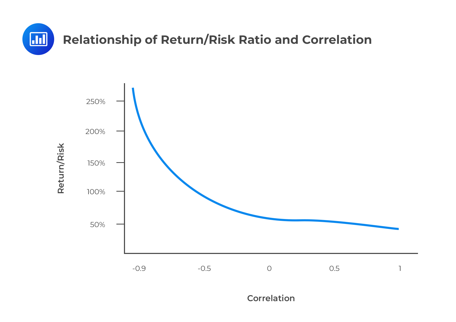
The figure below shows the impact of correlation on the portfolio return-risk ratio.
The lower the correlation between the two assets, the higher the return/risk ratio. A very high negative correlation (e.g., -0.95) results in a return/risk ratio greater than 250%. Avery high positive correlation (e.g., +0.95) results in a return/risk ratio near 50%.
Correlation of assets was a major contributor to the chaos and financial turmoil that rocked the financial world in 2007/2009. While there were multiple causes of the crisis, here are the main ones:
A benign Economic Environment That Fueled Speculation and Loose Credit Standards:
The period between 2003 and 2006 was marked by a benign economic environment with record levels of low credit spreads, low-interest rates, and low volatility. This had the effect of increasing risk-taking and speculative behavior among individual traders and institutions.
Complex Credit Products:
In the run-up to the crisis, multiple complex products were introduced in the market. Many of them were in the form of securitized assets such as collateralized debt obligations and constant-proportion debt obligations. Some of the largest financial institutions in the world became heavily involved in this new market but without a robust understanding of the attendant risks, particularly the correlation between the new assets and traditional products.
Model Risk:
Many investors put their trust in the new copula correlation model to model the correlation between structured assets. However, contrary to their expectations, the model itself resulted in complex computations that would have necessitated huge investments in research and analysis. For instance, most CDOs comprised of 125 assets. According to the model, this meant that there were 125(125−1)/2=7,750 asset correlation pairs to manage.
Moral Hazards:
Loose credit standards encouraged unqualified borrowers to seek credit in spite of their awareness that they would struggle to pay back the borrowed funds. And because the market was seemingly lucrative for banks, most of them turned a blind eye to warning signs such as the VaR. In fact, banks would recruit and remunerate rating agencies to assess the credit quality of various assets. By so doing, rating agencies compromised their independence and had an incentive to provide unduly positive ratings so as to keep their clients happy. Such favorable ratings gave the illusion of little price and default risk.
Increment of the Correlation between CDO Tranches:
Correlations between the tranches of the CDOs also increased during the crisis. The super-senior tranches were particularly hit, with most forcing sudden rating downgrades. It was not unusual to find a CDO having lost as much as 20% of its value in less than a week. As a result, several hedge funds (e.g., Marin Capital, Aman Capital) filed for bankruptcy.
Correlation trading refers to the trading of assets whose prices are, at least in part, informed by the co-movement of one or more assets in time. Traders often forecast changes in correlation in an attempt to make a financial gain.
Multi-asset options, also called rainbow options, present the most common way to trade correlation. The payoff of multi-asset options depends, at least partially, on the correlation between two or more underlying assets in the option. They are popular since they allow trading of not only volatility but also correlation. They are especially popular hedging tools for large entities with complex positions spread out across a range of classes. Below is a list of popular multi-asset correlation strategies along with their payoffs.
Definitions:
\(S_1\) = Price of asset one.
\(S_2\) = Price of asset two.
\(K\) = Strike price.
$$ \begin{array}{l|c} \textbf{Option} & \textbf{Payoff at maturity} \\ \hline \text{Option on the better of two} & {\text{Max}(S_1,S_2)} \\ \hline \text{Option on the worse of two} & {\text{Min}(S_1,S_2)} \\ \hline \text{Call on the maximum of two} & { \text{Max}[0, \text{Max}(S_1,S_2) – K] } \\ \hline \text{Exchange option} & {\text{Max}[0, S_2-S_1] } \\ \hline \text{Spread call option} & {\text{Max}[ 0, (S_2-S_1) – K]} \\ \hline \text{Option on the better of two or cash} & { \text{Max}(S_1,S_2, \text{cash}) } \\ \hline \text{Dual strike call option} & {\text{Max}[0, S_1-K_1, S_2-K_2} \\ \hline \text{Basket option} & { [\sum_{i=1}^n n_i S_i-K,0] } \\ {} & { \text{where } n_i \text{ is} } \\ {} & \text{the weight of asset S}\end{array} $$
In the list above, the lower the correlation, the higher the option price, with the exception of the option on the worse of two and the basket option.
Here are brief notes on a few of these options:
A quanto option is a cash-settled, cross-currency derivative, where the underlying asset is denominated in a currency other than the currency in which the option is settled. In other words, the underlying is in one currency, say, the dollar, but the option itself is settled in another currency, say, the Euro, at some fixed exchange rate.
If an investor has reasons to believe that a certain asset will do well in a certain country but has fears that the country’s currency might not perform as well, it would be advisable for the investor to buy an option in the foreign asset while keeping the payout in the home currency.
In the case of price Quanto options, the correlation between assets and currency exchange rates must be considered. The more positive the correlation coefficient, the lower the price for the quanto option. The lower the correlation coefficient, the more expensive the quanto option.
Note: The term Quanto is derived from the word quantity, meaning the amount that is re-exchanged for the home currency is unknown since it depends on the payoff of the option. This also explains why the Quanto options are sometimes called quantity-adjusting options.
A correlation swap is used to trade a fixed correlation between two or more assets with the correlation that actually occurs. It is a pure correlation play; it does not involve the price or volatility components of an underlying instrument. One party pays a fixed correlation rate in exchange for a realized, stochastic correlation rate. The realized correlation is the correlation between the assets that occurs during the time of the swap. Naturally, the fixed-rate payer is buying correlation, while the fixed-rate receiver is selling the correlation.
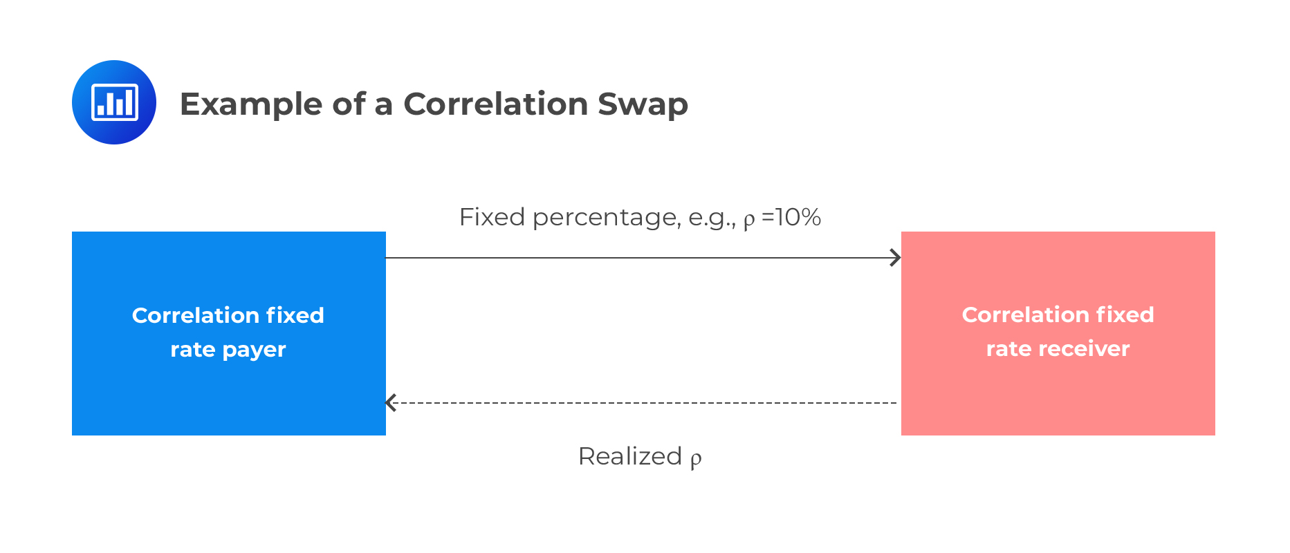 The payoff of a correlation swap for the correlation fixed rate payer at maturity, if N is the notional amount is:
$$ \text{Payoff} =\text N(\rho_{\text{realized}}-\rho_{\text{fixed}} ) $$
The realized correlation is computed as the average correlation between the assets in the correlation swap:
$$ \rho_{\text{realized}}=\cfrac { \sum_{i > j} w_i w_j \rho_{ij} }{ \sum_{i > j} w_i w_j } $$
Where \(\rho_{ij}\) is the pearson correlation coefficient between assets i and j. In this case, the formula for the realized correlation simplifies to:
$$ \rho_{\text{realized}}=\cfrac {2}{n^2-n} \sum_{i>j} \rho_{ij} $$
Assume that a correlation swap buyer pays a fixed correlation rate of 0.15 with a notional value of $10 million for one year for a portfolio of three assets. The realized pairwise correlations of the daily log returns [ln(St/St-1)] at maturity for the three assets are \(\rho_{21}= 0.6\), \(\rho_{31}= 0.3\), and \(\rho_{32}= 0.05\). What is the correlation swap buyer’s payoff?
First, we determine the value of the realized correlation:
$$ \begin{align*} \rho_{\text{realized}} & =\cfrac {2}{n^2-n} \sum_{i>j} \rho_{ij} \\& =\cfrac {2}{3^2-3} [0.6+0.3+0.05] \\ & =0.3167 \\ \end{align*} $$
Next, we now calculate the payoff:
$$ \text{Payoff} = N(\rho_{\text{realized}}-\rho_{\text{fixed}} ) = 10(0.3167 – 0.15) = $1,667,000 $$
Buying call options on an Index and selling call options on individual components:
There is a positive relationship between correlation and volatility. if correlation increases between stocks making up the index, the implied volatility of call options (on the index) will also increase. The increase in price for the index call options is expected to be greater than the increase in price for individual stocks that have a short call position.
Example: Buying a call option on the S&P 500 index and selling call options on individual stocks of the S&P 500 is a way of buying correlation.
Paying fixed in a variance swap on an index and receiving fixed on individual components:
This works much like buying a call on an index and selling a call on the individual components. An increase in correlation for securities within the index causes the variance to increase. As a result, the present value for the variance swap buyer, the fixed variance swap payer, will increase. This increase usually outperforms the potential losses from the short variance swap positions on the individual components.
The overall goal of any risk management process is to mitigate the main types of risk – market risk, credit risk, and operational risk. Other risk types include systemic risk, liquidity risk, volatility risk, and correlation risk. As established across the FRM curriculum, one of the most important risk measures is the value at risk (VaR). It helps us measure the potential loss in value over a given time interval, say, a month, with a specified degree of confidence.
The value at risk of a portfolio is given as:
$$ \text{VaR}_\text P=\sigma_\text P \alpha \sqrt {x} $$
where:
The volatility of portfolio, \(\sigma_P\), includes the correlation between assets in the portfolio. We can compute its value as follows:
$$ \sigma_P=\sqrt { \beta_h C\beta_V } $$
where:
An investor holds a two-asset portfolio with $20 million in asset A and $10 million in asset B. The portfolio correlation is 0.7, and the daily standard deviation of returns for assets A and B are 1.8% and 2.2%, respectively. What is the 10-day VaR of this portfolio at a 95% confidence level (i.e., \(\alpha\) = 1.645)?
Step 1: Construct the variance covariance matrix.
Since we have only two assets, we shall have a 2 × 2 matrix that will take the following shape:
$$ \begin{bmatrix} Cov(1,1) & Cov(1,2) \\ Cov(2,1) & Cov(2,2) \end{bmatrix} $$
(We use “1” to represent asset A and “2” to represent asset B for convenience)
Remember that:
$$ \begin{align*} \text{Cov}(X,X) & = \text{Var}(X); \\ \text{Cov}(X,Y) & = \text{Cov}(Y,X); \text{ and } \\ \text{Cov}(X,Y) & = \rho_{XY} × \sigma_X×\sigma_Y \\ \end{align*} $$
Therefore,
$$ \begin{align*} \text{Cov}(1,1) & =\sigma_1^2=0.018^2=0.000324; \\ \text{Cov}(2,2) & =\sigma_2^2=0.022^2=0.000484; \\ \text{Cov}(1,2) & = \text{Cov}(2,1) = 0.7×0.018×0.022=0.0002772; \\ \end{align*} $$
As such, our covariance matrix is:
$$ \begin{bmatrix} 0.000324 & 0.0002772 \\ 0.0002772 & 0.000484 \end{bmatrix} $$
Step 2: Determine the standard deviation of the portfolio.
We do this by first solving \(\beta_h C\), followed by \(\beta_h C)\beta_V\), and then finding the square root.
$$ \begin{align*} \beta_h C & =\left[ \begin{matrix} 20 & 10 \end{matrix} \right] \begin{bmatrix} 0.000324 & 0.0002772 \\ 0.0002772 & 0.000484 \end{bmatrix} \\ & = \left[ \begin{matrix} 20×0.000324+10×0.0002772 & 20×0.0002772+10×0.000484 \end{matrix} \right] \\ & = \left[ \begin{matrix} 0.009252 & 0.010384 \end{matrix} \right] \\ (\beta_h C)\beta_V & =\left[ \begin{matrix} 0.009252 & 0.010384 \end{matrix} \right] \begin{bmatrix} 20 \\ 10 \end{bmatrix} \\ & =0.009252×20+0.010384×10 \\ & =0.2889 \\ \end{align*} $$ Therefore, $$ \sigma_P=\sqrt { \beta_h C \beta_V }=\sqrt {0.2889} =0.5375 $$
Step 3: Compute the VaR.
$$ \text{VaR}_P=\sigma_P \alpha \sqrt {x}=0.5375×1.645×\sqrt {10}=2.7960 $$
Interpretation: The VaR estimate suggests that loss will only exceed $2,796,000 on 5 occasions for every 100 10-day periods. This is approximately 5 times every 1,000 trading days or 5 times every four years assuming there are 250 trading days in a year.
Bottom line:
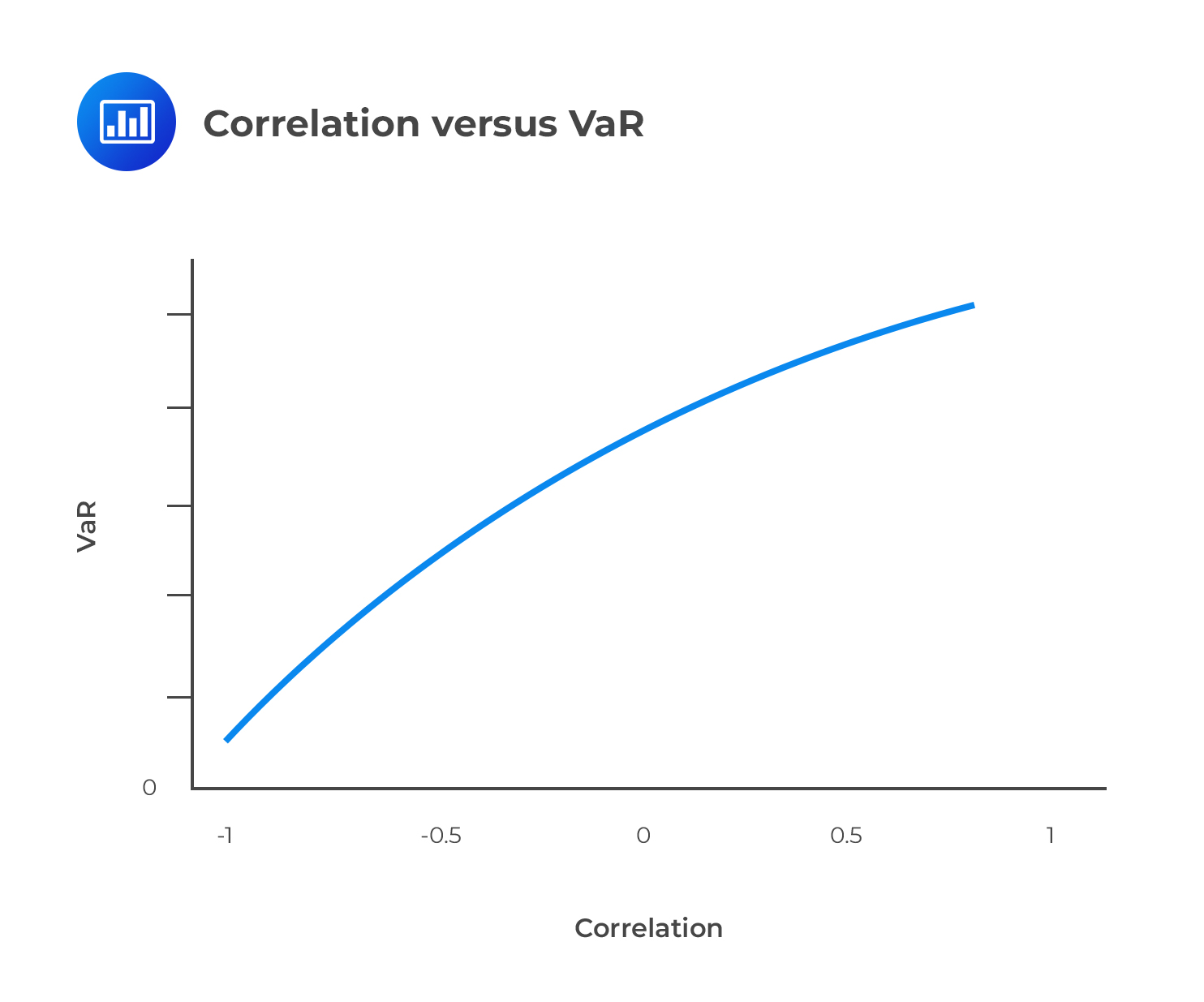
Correlation has a strong effect on the VaR of a portfolio. The lower the correlation, the lower the risk (as measured by VaR). Negative correlation is always preferred because it implies that when the value of one asset decreases, the value of the other asset, on average, increases. Hence, a negative correlation reduces the overall risk of the portfolio.
The relationship between VaR and correlation can be represented by an upward sloping curve:
 Regulation and Correlation
Correlation forms a critical part of regulatory models that have been developed over the years in an attempt to better monitor risk positions. This can be seen in Basel accords which mainly apply to banks. Basel I, II, and III are regulatory guidelines designed to ensure the stability of the banking system. As the latest of these, Basel III is being developed to address the deficiencies brought to the fore during the 2007/2008 financial crisis. Some of the issues being looked at include:
It is important to note that The Basel Committee on Banking Supervision currently requires banks to hold capital for assets in the trading book of at least three times greater than 10-day VaR.
Correlation risk is closely related to systemic risk and it plays an important role in the management of market and credit risks which constitute the main types of financial risk.
Comprising of equity risk, interest rate risk, currency risk, and commodity risk, market risk is greatly influenced by correlation risk. Market risk is measured using VaR. The concept of VaR is typically applied to market risk measurement since it has, as an input, the covariance matrix of assets in a portfolio. This means it implicitly incorporates correlation risk. For extreme events, Expected Shortfall (also termed conditional VaR or tail risk) will also measure the market risk just like VaR. A thorough ES valuation will naturally include the correlation between asset returns in a portfolio.
Credit risk is comprised of migration risk and default risk.
Migration risk is occasioned by a decline in a debtor’s credit quality. Worsening credit quality is usually accompanied by a decline in asset prices. Such a development hurts a creditor. A bond investor who has hedged their investment with a CDS is exposed to the correlation between the reference asset and the counterparty, the CDS seller. Increased correlation leads to a paper loss for the investor. In fact as correlation increases, so does the probability of a total loss of the investment.
Default correlation is the degree to which defaults occur together. To reduce default correlation risk, it is advisable for lenders to have a loan portfolio that is sector diversified since default correlation within sectors is higher than between sectors.
Systemic risk is attributed either to the collapse of a financial market or an entire financial system. To find an example, we only need to look back at 2008 when the entire credit market collapsed. These financial failures will typically spread to the economy leading to a GDP decrease, increased unemployment, and consequently, reduced living standards. There is an interdependence between systemic risk and correlation. A systemic decline in stocks will sharply increase correlations between stocks.
Concentration risk is the risk of financial loss due to a concentrated exposure to a particular group of counterparties. Concentration risk can be quantified in the form of the concentration ratio. A lower (higher) concentration ratio indicates that a creditor has more (less) diversified default risk. For example, for an investor with 10 loans of equal size extended to 10 different borrowers, the concentration risk is 1/10 = 0.1. But if the investor just has a single loan extended to a single borrower, the concentration ratio would be 1/1 = 1.
A commercial bank extends a $10 million loan to company X, which has a 5% default probability. What are the concentration ratio and expected loss (EL) for the bank under the worst-case scenario? Assume loss given default (LGD) is 100%.
Since there is only one borrower, the concentration risk is 1.
In the worst-case scenario, a default event by X results in a total loss of loan value. Given that there is a 5% probability that company X defaults, EL for the bank is \($500,000 (= 0.05 x 10,000,000).\)
This time, let’s assume that bank X extends two loans: a $5 million loan to A and a similar amount to B. Let’s assume further that A and B each have a 5% default probability. What is the concentration ratio? What will be the impact on the expected loss (EL) for the bank under the worst-case scenario? Assume the default correlation between companies is bigger than 0 and smaller than 1.
The bank’s concentration ratio is reduced to ½. Since the default correlation between X and Y is bigger than 0 and smaller than 1, the worst-case scenario [i.e., the default of X and Y, P(\(X\cap Y\)), with a loss of $500,000 is reduced. This can be seen in the figure below:
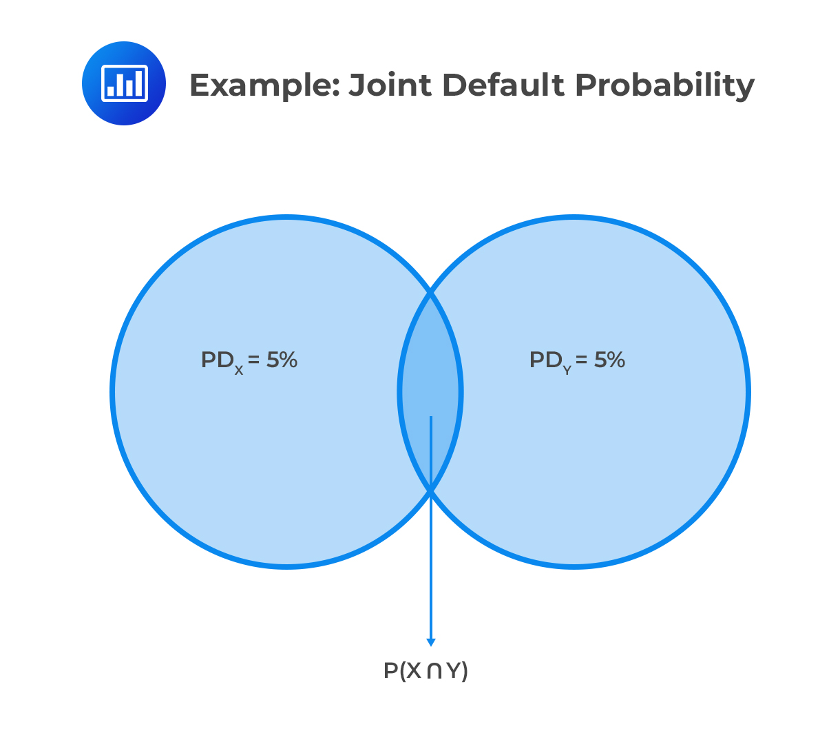 The exact joint default probability \(P(X \cap Y)\) depends on the correlation model and correlation parameter values.
If the default correlation between X and Y is 1.0, the expected loss for the bank is $500,000 (0.05 x $10,000,000). In such a case, there is no benefit from the lower concentration ratio. It would be the same as extending a $10 million loan to one company.
If we further decrease the concentration ratio (by extending loans to more borrowers), the worst-case scenario (i.e., the expected loss of 5%) decreases further.
The defaults of companies X and Y are expressed as two binomial variables; they take the value 1 if in default, and 0 if they are not. The joint probability of default for the two binomial events is:
$$ P(X \cap Y)=\rho_{XY} \sqrt{ P_X (1-P_X)P_Y (1-P_Y) } +P_X P_Y $$
where:
Question 1
Calculate the payoff of a correlation swap if assets are 3 and the realized pairwise correlations of the log returns at maturity level are given as 0.95, 0.81 and 0.54. You are also given that the notational amount is $10 million at a 15% fixed rate and 1-year maturity.
- $6.17 million.
- $3.61 million.
- $13.8 million.
- $7.67 million.
The correct answer is A.
The realized correlation is calculated as:
$$ { \rho }_{ realized }=\frac { 2 }{ { n }^{ 2 }-n } { \Sigma }_{ i>j }{ \rho }_{ i,j } $$
Therefore, we have:
$$ { \rho }_{ realized }=\frac { 2 }{ 3^{ 2 }-3 } \left( 0.54+0.81+0.95 \right) =0.7667 $$
Following the equation:
$$ N\left( { \rho }_{ realized }-{ \rho }_{ fixed } \right) $$
\(\Rightarrow \)The payoff of the correlation fixed rate player at maturity is
$$ \text{\$10 million} \times \left( 0.7667–0.15 \right) =$6.17 \text{Million} $$
Question 2
Assume that institution \(X\) has a historical default probability of \(P\left( X \right) =7\% \) and that company \(Y\) has historical default probability of \(P\left( Y \right) =5\% \). What is their joint historical default probability if \(P\left( X \right) \) and \(P\left( Y \right) \) are independent?
- 0.35%.
- 35%.
- 58.33%.
- 5.83%.
The correct answer is A.
Remember that events \(A\) and \(B\) are independent if their joint probabilities equal the product of their individual probabilities:
$$\begin{align*} P\left( A\cap B \right) &=P\left( A \right) P\left( B \right)\\ P\left( X\cap Y \right)& =0.35\% \end{align*}$$
But:
$$ P\left( A \right) =\frac { P\left( A\cap B \right) }{ P\left( B \right) } $$
And:
$$ P\left( B \right) =\frac { P\left( A\cap B \right) }{ P\left( A \right) } =P\left( B|A \right) $$
Therefore:
$$ P\left( X \right) =\frac { 0.35\% }{ 5\% } =7\% $$
And:
$$ \begin{align*}P\left( Y \right)& =\frac { 0.35\% }{ 7\% } =5\% \\ \Rightarrow P\left( X\cap Y \right) &=P\left( X \right) P\left( Y \right) \end{align*}$$
Since:
$$ 0.35\%=7\%\times 5\% $$
Prepare for FRM exams with structured study materials, guided learning, and focused practice across market risk and correlation risk topics.
Offered by AnalystPrep


Get Ahead on Your Study Prep This Cyber Monday! Save 35% on all CFA® and FRM® Unlimited Packages. Use code CYBERMONDAY at checkout. Offer ends Dec 1st.