Expectations, Risk Premium, Convexity, and the Shape of the Term Structure

After completing this reading, you should be able to:

• Explain the role of interest rate expectations in determining the shape of the term structure.
• Apply a risk-neutral interest rate tree to assess the effect of volatility on the shape of the term structure.
• Estimate the convexity effect using Jensen’s inequality.
• Identify the components into which the return on a bond can be decomposed, and calculate the expected return on a bond for a risk-averse investor.

This chapter explains the role of interest rate expectation in determining the shape of the term structure. It shows how spot or forward rates are determined by expectations of future short-term rates, the volatility of short-term rates and an interest rate premium.

Role of Interest Rate Expectations in Determining the Shape of the Term Structure

Expectations imply uncertainty. For example, an investor might expect the one-year rate next year to be, say, 10%, but they know very well that the actual rate might fall short or even be slightly higher.

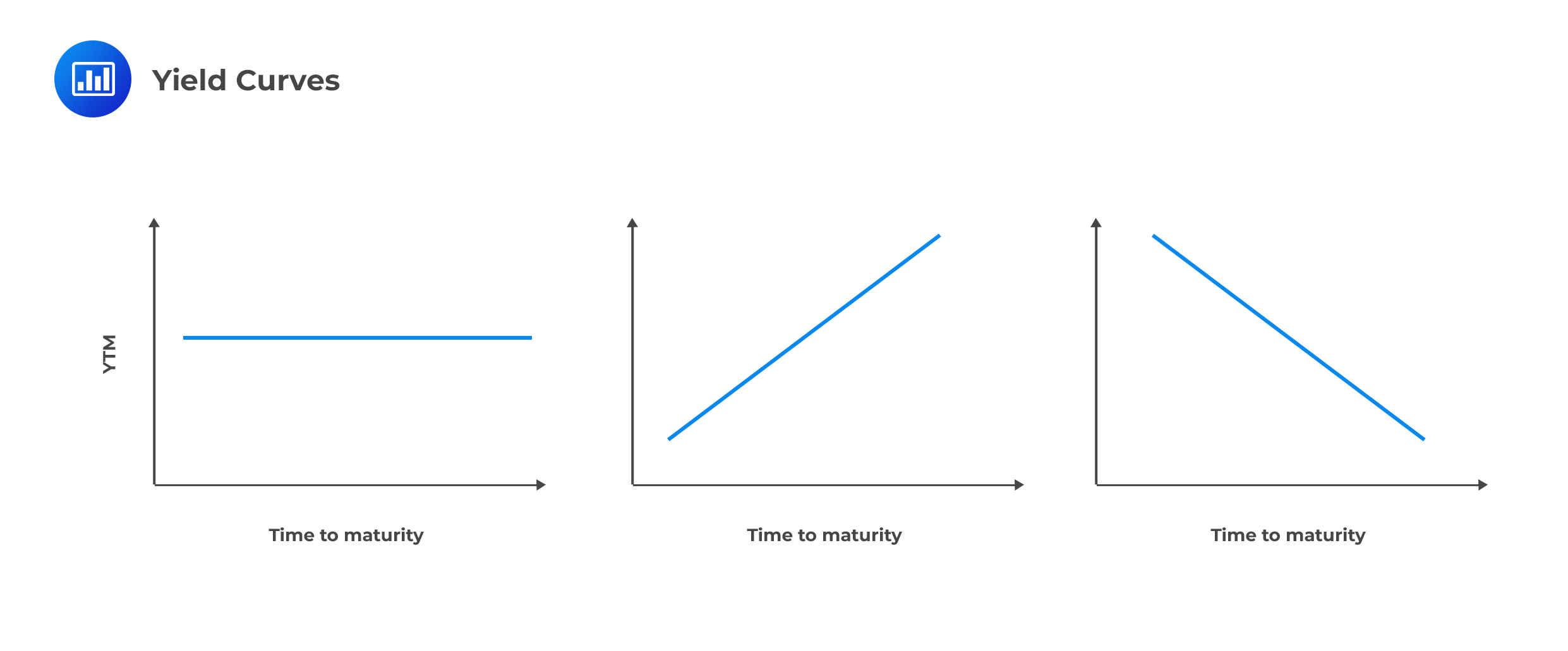
Expectations among investors have a major bearing on the shape of the term structure of interest rates. The resulting yield curve can be flat, upward sloping, or downward sloping.

Illustrative example:

Part 1

Assume that the 1-year interest rate is 6% and investors have estimated the future 1-year forward rates at 6% for the next two years. Given these interest rate expectations, the price (present values) of 1-, 2-, and 3-year zero-coupon bonds per $1 face value assuming annual compounding are calculated as follows:

$$ \begin{align*} \text{Price of 1-year zero} & =\cfrac {$1}{1.06}=$0.9434 \\ \text{Price of 2-year zero} & =\cfrac {$1}{(1.06)(1.06)}=$0.8900 \\ \text{Price of 3-year zero} & =\cfrac {$1}{(1.06)(1.06)(1.06)}=$0.8696 \\ \end{align*} $$

In summary, investors expect the 1-year spot rates to be 6% for the next three years. What’s the implication? The yield curve is flat. Investors would be willing to lock in interest rates for two or three years at 6% by purchasing, say, a three-year bond with an annual coupon of 6%. The 1-year, 2-year, and 3-year spot rates are all equal.

Part 2

Now, assume that the 1-year spot rate remains at 6%, but investors expect the 1-year rate in a year’s time to be 8%, and the 1-year rate to be 10% in two years. In this case, the 2-year and 3-year spot rates will not be 10%. The 2-year spot rate, \(\hat r\)(2), will be 7%, calculated as follows:

$$ \text{Price of 2-year zero} =\cfrac {$1}{(1.06)(1.08)}=\cfrac {1}{(1+{\hat r}(2))^2 }; \hat r(2)= 0.07 $$

Similarly, the 3-year spot rate, \(\hat r\)(3), will be 7.99%, calculated as follows:

$$ \text{Price of 3-year zero} =\cfrac {$1}{(1.06)(1.08)(1.1)}=\cfrac {1}{(1+r ̂(3))^3 }; r ̂(3)= 0.0799 $$

In a nutshell, investors expect the 1-year spot rate to be 6%, the 2-year spot rate to be 7%, and the 3-year spot rate to be 7.99%. What’s the implication? The yield curve is upward sloping. Would investors be willing to lock in an interest rate of 6% for two or three years? No.

Part 3

Now, assume that the 1-year spot rate remains at 6%, but investors expect the 1-year rate in a year’s time to be 4%, and the 1-year rate to be 2% in two years’ time. In this case, the 2-year and 3-year spot rates will be different, again. The 2-year spot rate, \(\hat r\)(2), will be 5%, calculated as follows:

$$ \text{Price of 2-year zero} =\cfrac {$1}{(1.06)(1.04)}=\cfrac {1}{(1+{\hat r} (2))^2} ; {\hat r}(2)= 0.05 $$ Similarly, The 3-year spot rate, \({\hat r}\)(3), will be 3.99%, calculated as follows: $$ \text{Price of 3-year zero}=\cfrac {$1}{(1.06)(1.04)(1.2)}=\cfrac {1}{(1+r ̂(3))^3} ;{\hat r}(3)= 0.0399 $$

In summary, investors expect the 1-year spot rate to be 6%, the 2-year spot rate to be 5%, and the 3-year spot rate to be 3.99%. What’s the implication? The yield curve is downward sloping. And unlike in the upward sloping case, investors would have an incentive to lock in an interest rate of 6% for two or three years.

Bottom line:

Interest rate expectations inform the shape and level of the term structure for short-term horizons. However, investors have much less confidence in their expectations about spot rates several periods into the future. Therefore, expectations are unable to describe the shape of the term structure for long-term horizons. This is because future expectations must factor in inflationary tendencies.

Applying a Risk-neutral Interest Rate Tree to Assess the Effect of Volatility on the Shape of the Term Structure

Using a risk-neutral interest rate tree, it is possible to demonstrate that when there is uncertainty regarding expected rates, the volatility of expected rates causes the future spot rates to be lower.

Illustrative Example:

Assume that the following tree gives the true process for the one-year rate:

$$ \begin{array} {} & {} & {} & {\scriptsize { 1 }/{ 2 } } & 10\% \\ {} & {} & 8\% & {\Huge \begin{matrix} \diagup \\ \diagdown \end{matrix} } & {} \\ 6\% & {\begin{matrix} \scriptsize { 1 }/{ 2 } \\ \begin{matrix} \begin{matrix} \quad \quad \quad \Huge \diagup \\ \end{matrix} \\ \quad \quad \quad \Huge \diagdown \end{matrix} \\ \scriptsize { 1 }/{ 2 } \end{matrix} } & {} & {\scriptsize \begin{matrix} \begin{matrix} { 1 }/{ 2 } \\\scriptsize \begin{matrix} \\ \end{matrix} \end{matrix} \\ \begin{matrix} \\ \end{matrix} \\ { 1 }/{ 2 } \end{matrix} }& 6\% \\ {} & {} & 4\% & {\Huge \begin{matrix} \diagup \\ \diagdown \end{matrix} } & {} \\ {} & {} & {} & {\scriptsize { 1 }/{ 2 }} & 2\% \\ \end{array} $$ $$ \begin{array} \\ \text{Year 0} & {} & {} & {} & \text{Year 1} & {} & { } & {} & \text{Year 2} \\ \end{array} $$

The expected interest rate on year 1 is .5 × 8% + .5 × 4% or 6% and that the expected rate on year 2 is .25 × 10% + .5 × 6% + .25 × 2% or 6%.

The price of a one-year zero is, by definition, 1/1.06 or .9434, implying a one-year spot rate of 6%.

Under the assumption of risk-neutrality, the price of a two-year zero may be calculated by discounting the terminal cash flow using the preceding interest rate tree:

$$ \begin{array} {} & {} & {} & {\scriptsize { 1 }/{ 2 } } & 1 \\ {} & {} & 0.9259 & {\Huge \begin{matrix} \diagup \\ \diagdown \end{matrix} } & {} \\ 0.8903 & {\begin{matrix} \scriptsize { 1 }/{ 2 } \\ \begin{matrix} \begin{matrix} \quad \quad \quad \Huge \diagup \\ \end{matrix} \\ \quad \quad \quad \Huge \diagdown \end{matrix} \\ \scriptsize { 1 }/{ 2 } \end{matrix} } & {} & {\scriptsize \begin{matrix} \begin{matrix} { 1 }/{ 2 } \\\scriptsize \begin{matrix} \\ \end{matrix} \end{matrix} \\ \begin{matrix} \\ \end{matrix} \\ { 1 }/{ 2 } \end{matrix} }& 1 \\ {} & {} & 0.9615 & {\Huge \begin{matrix} \diagup \\ \diagdown \end{matrix} } & {} \\ {} & {} & {} & {\scriptsize { 1 }/{ 2 }} & 1 \\ \end{array} $$ $$ \begin{array} \\ \text{Year 0} & {} & {} & {} & {} & \text{Year 1} & {} & { } & { } & {} & \text{Year 2} \\ \end{array} $$

$$ \left[0.5 x \left( \frac {$0.9259}{1.06} \right) \right] + \left[0.5 x \left( \frac {$0.9615}{1.06} \right) \right] = $0.8903 $$

Hence, the two-year spot rate, \(\hat r\)(2) is 5.9819%, calculated as follows:

$$ \begin{align*} 0.8903 & = \cfrac {1}{\left(1+\hat r(2) \right)^2} \\ 0.8903(1+\hat r(2))^2 & =1 \\ (1+\hat r(2))^2 & =1.1232 \\ \hat r (2) & =1.059819-1 =0.059819 \\ \end{align*} $$

We can see that even though the one-year rate is 6% and the expected one-year rate in one year is 6%, the two-year spot rate is 5.9819%. This affirms the fact that when there is uncertainty regarding expected rates, the volatility of expected rates causes the future spot rates to be lower.

The 1.8-basis point difference between the spot rate that would obtain in the absence of uncertainty, 6%, and the spot rate in the presence of volatility, 5.9819%, is the effect of convexity on that spot rate.

Estimating the Convexity Effect Using Jensen’s Inequality

The convexity effect arises from a special case of Jensen’s Inequality:

$$ E \left[ \cfrac {1}{[1+r]} \right]>\cfrac {1}{E[1+r]} $$

Example: Applying Jensen’s Inequality

Assume that next year the 1-year spot rate will be 8% or 4% with equal (0.5) probability. Demonstrate Jensen’s inequality for a 2-year zero-coupon bond with a face value of $1, assuming that the previous interest rate expectations apply (shown below for convenience).

$$ \begin{array} {} & {} & {} & {\scriptsize { 1 }/{ 2 } } & 10\% \\ {} & {} & 8\% & {\Huge \begin{matrix} \diagup \\ \diagdown \end{matrix} } & {} \\ 6\% & {\begin{matrix} \scriptsize { 1 }/{ 2 } \\ \begin{matrix} \begin{matrix} \quad \quad \quad \Huge \diagup \\ \end{matrix} \\ \quad \quad \quad \Huge \diagdown \end{matrix} \\ \scriptsize { 1 }/{ 2 } \end{matrix} } & {} & {\scriptsize \begin{matrix} \begin{matrix} { 1 }/{ 2 } \\\scriptsize \begin{matrix} \\ \end{matrix} \end{matrix} \\ \begin{matrix} \\ \end{matrix} \\ { 1 }/{ 2 } \end{matrix} }& 6\% \\ {} & {} & 4\% & {\Huge \begin{matrix} \diagup \\ \diagdown \end{matrix} } & {} \\ {} & {} & {} & {\scriptsize { 1 }/{ 2 }} & 2\% \\ \end{array} $$ $$ \begin{array} \\ \text{Year 0} & {} & {} & {} & \text{Year 1} & {} & { } & {} & \text{Year 2} \\ \end{array} $$

Solution

The left-hand side of Jensen’s inequality is the expected price in one year using the 1-year spot rates of 8% and 4%.

$$ E \left[\cfrac {$1}{(1+r)}\right]=0.5×\cfrac {$1}{1.08}+0.5×\cfrac {$1}{1.04}=$0.9437 $$ The expected price in one year using an expected rate of 6 % computes the right-hand side of the inequality as follows: $$ \cfrac {1}{E[1+r]} =\cfrac {$1}{0.5×1.08+0.5×1.04}=\cfrac {$1}{1.06}=0.9434 $$

Therefore, the left-hand side is greater than the right-hand side, $0.9437 > $0.9434.

If the current 1-year rate is 6%, the price of a 2-year zero-coupon bond is determined by dividing each side of the equation by 1.06. Therefore, the price of the 2-year zero-coupon bond on the left-hand side of Jensen’s inequality equals $0.8903 (calculated as $0.9437/1.06). The right-hand side is calculated as the price of a 2-year zero-coupon bond discounted for two years at the expected rate of 6%, which yields $0.8900 (calculated as $1/1.06²).

This effectively demonstrates that the price of the 2-year zero-coupon bond is greater than the price obtained by discounting the $1 face amount by 6% over the first period and by 6% over the second period. As a result, we know that since the 2-year zero-coupon price is higher than the price achieved through discounting, its implied rate must be lower than 6%.

Decomposition of Bond Returns and Expected Return for Risk-Averse Investors

Components of Bond Return Decomposition

The return on a bond can be broken down into three primary components:

Expected Return Component:

• Represents the return an investor expects to earn if interest rates remain constant.
• Typically calculated as the yield to maturity (YTM) of the bond.

Duration Effect:

• Captures the bond price’s sensitivity to interest rate changes.
• Mathematically, duration (D) measures the percentage change in bond price for a 1% change in interest rates.
• When interest rates rise, bond prices fall, and vice versa.

Convexity Effect:

• Accounts for the non-linear relationship between bond prices and interest rates.
• Bonds with higher convexity experience smaller losses when rates rise and greater gains when rates fall.
• Mathematically, convexity (C) is the second derivative of bond price with respect to interest rates.

Using Itô’s Lemma, the decomposition of the instantaneous bond return can be represented as:

$$\frac{dP}{P}= f(t)dt – Ddr + \frac{1}{2}C \sigma^2 dt$$

Where:

• \(f(t)dt\) is the expected return component,
• \(Ddr\) represents the impact of duration,
• \(\frac{1}{2}C \sigma^2 dt\) accounts for convexity.

Expected Return for Risk-Averse Investors

In a risk-neutral world, investors do not require a risk premium. Instead, they expect returns to align with the risk-free rate. Under risk neutrality, the expected return on a bond is given by:

$$E\left[ \frac{dP}{P} \right] = rdt$$

However, in reality, most investors are risk-averse and require additional compensation for taking on interest rate risk. The expected return equation for risk-averse investors incorporates a risk premium \(\lambda\), which accounts for the uncertainty in interest rate movements and its impact on bond prices.

Mathematically, for a risk-averse investor:

$$E\left[ \frac{dP}{P} \right] = rdt + \lambda Ddt$$

Where:

• \(rdt\) represents the risk-free rate (or short-term rate of interest),
• \(\lambda Ddt\) represents the risk premium, which is proportional to duration.

Interpretation of Risk Premium and Sharpe Ratio

The risk premium is directly linked to the bond’s duration and volatility. A bond with a higher duration will demand a higher risk premium.

One way to analyze the risk premium is through the Sharpe Ratio (SR):

$$ SR = \frac{E\left(\frac{dP}{P}\right)-rdt}{\sigma Ddt} = \frac{\lambda}{\sigma}$$

Where:

• \(E\left(\frac{dP}{P}\right)\) is the expected excess return of the bond,
• \(r_0 dt\) is the short-term risk-free rate,
• \(\sigma\) is the standard deviation of returns,
• \(D\) represents the duration of the bond,
• \(\lambda\) is the risk premium, measuring compensation for taking interest rate risk.

The Sharpe ratio provides insight into how compensation for risk changes with duration. Since the standard deviation of the return is given by the duration times the standard deviation of interest rate changes, the Sharpe ratio remains an important metric for evaluating risk-adjusted performance. A higher Sharpe ratio indicates better risk-adjusted returns.

Example: Incorporating a Risk Premium

Suppose the following interest rate tree exists:

$$ \begin{array} {} & {} & {} & {\scriptsize { 1 }/{ 2 } } & 10\% \\ {} & {} & 8\% & {\Huge \begin{matrix} \diagup \\ \diagdown \end{matrix} } & {} \\ 6\% & {\begin{matrix} \scriptsize { 1 }/{ 2 } \\ \begin{matrix} \begin{matrix} \quad \quad \quad \Huge \diagup \\ \end{matrix} \\ \quad \quad \quad \Huge \diagdown \end{matrix} \\ \scriptsize { 1 }/{ 2 } \end{matrix} } & {} & {\scriptsize \begin{matrix} \begin{matrix} { 1 }/{ 2 } \\\scriptsize \begin{matrix} \\ \end{matrix} \end{matrix} \\ \begin{matrix} \\ \end{matrix} \\ { 1 }/{ 2 } \end{matrix} }& 6\% \\ {} & {} & 4\% & {\Huge \begin{matrix} \diagup \\ \diagdown \end{matrix} } & {} \\ {} & {} & {} & {\scriptsize { 1 }/{ 2 }} & 2\% \\ \end{array} $$

A risk-neutral investor would value a 2-year zero coupon bond at $0.99437 per $1 face value, calculated as follows:

$$ \cfrac { \left( \frac {$1}{1.08} + \frac {$1}{1.04} \right)0.5 }{1.06}=$0.8903 $$

The price of $0.8903 implies a 1-year expected return of 6%. However, this is only the average return. The actual return will be either 4% or 8%. As a result, a risk-averse investor will demand a risk premium for bearing this interest rate risk, and demand a return greater than 6% for buying a 2-year zero-coupon bond and holding it for the next year.

Assume that a risk-averse investor demands a 30-basis point premium. To come up with the price of the 2-year zero-coupon bond would decrease to $0.8878, calculated as follows:

$$ \cfrac { \left( \frac {$1}{1.083} + \frac {$1}{1.043} \right)0.5 }{1.06}=$0.8878 $$

It follows that a risk-averse investor would be willing to pay much less for every $1 face value of the bond.

Question 1

Investors value the current one-year interest rate at 8.30%. If they also forecast that for the following year, the one-year interest rate will be 9.43%, then the two-year spot rate, \(\rho \left( 2 \right) \), is closest to:

1. 8.86%.
2. 9.43%.
3. 18.51%.
4. 9.26%.

The correct answer is A.

The two- year spot rate \(\rho \left( 2 \right) \) is such that:

$$ \begin{align*}{ P }^{ 2 }&=\frac { 1 }{ \left( 1.0830 \right) \left( 1.0943 \right) }=\frac { 1 }{ { \left( 1+\rho \left( 2 \right) \right) }^{ 2 } } \\ &\Rightarrow { \left( 1+\rho \left( 2 \right) \right) }^{ 2 }=\left( 1.0830 \right) \left( 1.0943 \right)\\ \rho \left( 2 \right)& =0.886=8.86\% \end{align*}$$

Question 2

Assume that the following tree gives the true process for the one-year rate.

$$ \begin{array} \hline {} & {} & {} & {\scriptsize 0.5 } & 22\% \\ {} & {} & 18.5\% & {\Huge \begin{matrix} \diagup \\ \diagdown \end{matrix} } & {} \\ 15\% & {\begin{matrix} \scriptsize 0.5 \\ \begin{matrix} \begin{matrix} \quad \quad \quad \Huge \diagup \\ \end{matrix} \\ \quad \quad \quad \Huge \diagdown \end{matrix} \\ \scriptsize 0.5 \end{matrix} } & {} & \scriptsize 0.5 & 15\% \\ {} & {} & 11.5\% & {\Huge \begin{matrix} \diagup \\ \diagdown \end{matrix} } & {} \\ {} & {} & {} & {\scriptsize 0.5} & 8\% \\ \end{array} $$

Compute the expected interest rate for dates 1 and 2, respectively.

1. Both are 15%.
2. 12% and 19%.
3. 18.5% and 11.5%.
4. 8% and 22%.

The correct answer is A.

The expected interest rate on date 1 is:

$$ 0.5\times 11.5+0.5\times 18.5=15\% $$

The expected interest rate for date 2 is:

$$ 0.25\times 22+0.5\times 15+0.25\times 8=15\% $$

Question 3

Using the data provided in the following tree, apply the Jensen’s inequality for estimation of connectivity to show why the 2-year spot rate is less than 15%.

$$ \begin{array} \hline {} & {} & {} & {\scriptsize 0.5 } & 22\% \\ {} & {} & 18.5\% & {\Huge \begin{matrix} \diagup \\ \diagdown \end{matrix} } & {} \\ 15\% & {\begin{matrix} \scriptsize 0.5 \\ \begin{matrix} \begin{matrix} \quad \quad \quad \Huge \diagup \\ \end{matrix} \\ \quad \quad \quad \Huge \diagdown \end{matrix} \\ \scriptsize 0.5 \end{matrix} } & {} & \scriptsize 0.5 & 15\% \\ {} & {} & 11.5\% & {\Huge \begin{matrix} \diagup \\ \diagdown \end{matrix} } & {} \\ {} & {} & {} & {\scriptsize 0.5} & 8\% \\ \end{array} $$

1. 0.853 > 0.657.
2. 0.798 > 0.713.
3. 0.758 > 0.756.
4. 0.658 > 0.456.

The correct answer is C.

According to the Jensen’s inequality:

$$\begin{align*} E\left[ \frac { 1 }{ 1+r } \right] &>\frac { 1 }{ E\left[ 1+r \right] }=\frac { 1 }{ 1+E\left[ r \right] }\\  \Rightarrow 0.5\times \frac { 1 }{ 1.185 } +0.5\times \frac { 1 }{ 1.115 } &>\frac { 1 }{ 0.5\times 1.185+0.5\times 1.115 } =\frac { 1 }{ 1.15 } \end{align*}$$

Dividing both sides by 1.15:

$$ \begin {align*}\Rightarrow \frac { 1 }{ 1.15 } \left[ 0.5\times \frac { 1 }{ 1.185 } +0.5\times \frac { 1 }{ 1.115 } \right]& >\frac { 1 }{ { 1.15 }^{ 2 } }\\ \Rightarrow 0.758 &> 0.756\end{align*} $$