Backtesting VaR

After completing this reading, you should be able to:

• • Describe backtesting and exceptions and explain the importance of backtesting VaR models.
  • Explain the significant difficulties in backtesting a VaR model.
  • Verify a model based on exceptions or failure rates.
  • Identify and describe Type I and Type II errors in the context of a backtesting process.
  • Explain the need to consider conditional coverage in the backtesting framework.
  • Describe the Basel rules for backtesting.

In this chapter, the accuracy of VaR models is verified by backtesting techniques. Backtesting is a formal statistical framework that verifies whether or not actual losses are in line with the projected losses. This is achieved by systematically comparing the history of VaR forecasts with their associated portfolio returns. VaR risk managers and users find these procedures, also called reality checks, very essential when checking that their VaR forecasts are well-calibrated.

What is Backtesting?

Backtesting is the process of comparing losses predicted by a value at risk (VaR) model to those actually experienced over the testing period. It is done to ensure that VaR models are reasonably accurate. Risk managers systematically check the validity of the underlying valuation and risk models by comparing actual to predicted levels of losses.

The overall goal of backtesting is to ensure that actual losses do not exceed the expected losses at a given level of confidence. Exceptions are the number of actual observations over and above the expected level. In the context of the VaR, the number of exceptions falling outside of the VaR confidence level should not exceed one minus the confidence level. For instance, exceptions should occur less than 1% of the time if the level of confidence is 99%. Exceptions are also called exceedances.

For a model that is perfectly calibrated, the number of observed exceptions should be approximately the same as the VaR significance level.

• When too many exceptions are observed, the model involved is not calibrated properly and actually underestimates risk. The regulator may respond by imposing fines and/or additional capital requirements so as to shield risk-taking units from possible financial strain.
• When too few exceptions are observed, this, again, can be a big problem. It would normally imply that the bank is not allocating funds to risk-taking units in an efficient manner. Such a scenario will put managers on a collision path with shareholders or investors.

Examples

• Over 100 days, a good 95.0% VaR model will produce approximately 5.0% * 100 days = 5 exceptions.
• Over 1,000 days, a good 99.0% VaR model will produce approximately 1.0% * 1,000 days = 10 exceptions.
• Assuming there are 252 trading days in a year, a 95.0% daily VaR should be exceeded by about 13 days per year; 5% * 252 days = 12.6 days.
• Assuming that there are 252 trading days in a year, a 99.0% daily VaR should be exceeded by about 10 days over a four-year period; 1% * 4 * 252 days = 10.08 days.

Backtesting is also important for the following reasons:

• Backtesting gives a “reality check” on whether VaR forecasts are properly calibrated or accurate. Too many exceptions should prompt a recalibration of the model and a thorough re-examining of assumptions, parameters, and the entire modeling process.
• Backtesting provides the Basel Committee with a critical evaluation technique to test the adequacy of internal VaR models.
• Backtesting helps bank regulators to verify risk models used by subject banks. The essence of backtesting is to identify banks using models that may potentially underestimate risk, thereby not only endangering the financial health of an individual bank but the industry in general (This is particularly true for systematically important banks, SIBs). It is not uncommon to find banks with excessive exceptions (more than four exceptions in a sample size of 250) being penalized with higher capital requirements.

Difficulties in Backtesting a VaR Model

There are several things that make backtesting a difficult task for risk managers.

To begin with, VaR models are based on static portfolios, but in reality, actual portfolio compositions are in a constant state of change to reflect daily gains or losses, expenses, and buy/sell decisions. For this reason, a risk manager should track both the actual portfolio return and the hypothetical (static) return. In some instances, it may also make sense to carry out backtesting using a “clean return” instead of the actual return. Clean return is actual return minus all non-mark-to-market items such as fees, commissions, and net income.

Moreover, the sample backtested may not be representative of the true underlying risk. Since the backtesting period is just a limited sample, it would be a stretch of reality to expect the predicted number of exceptions in every sample. At the end of the day, backtesting remains a statistical process with accept-or-reject decisions.

Verifying a Model Based on Exceptions or Failure Rates

For a model to be completely accurate, the number of exceptions would have to be the same as the VaR significance level. Note that in this case, significance is one minus the confidence level. We have already established that the backtesting period constitutes a limited sample at a specific confidence level. This means that it would be unrealistic to expect to find the model-predicted number of exceptions in every sample. In other words, there are instances where the observed number of exceptions will not be the same as that predicted by the model. Even then, remember that this does not necessarily mean that the model is flawed. As such, we must establish the level (point) at which we reject the model.

We verify a model by recording the failure rate, which represents the proportion of times VaR is exceeded in a given sample. Under the null hypothesis of a correctly calibrated model (Null \(\text H_0\): correct model), the number of exceptions (x) follows a binomial probability distribution:

$$ \text f(\text x) ={^{\text T}} \text C_{\text x} {\text P}^{\text x} (1-\text P)^{\text T-\text x} $$

Where T is the sample size and p is the probability of exception (p = 1 – confidence level).

The expected value of (x) is p*T and a variance, \(\sigma^2(x) = \text p*(1-\text p)*{\text T}\)

The inherent assumption here is that exceptions (failures) are independent and identically distributed (i.i.d.) random variables.

If we use N to represent the number of exceptions, the failure rate is given by N/T.

Example 1: Computing the Probability of Exceptions

What is the probability of observing x = 0 exceptions out of a sample of T = 250 observations when the true probability (p) is 1%?

Solution

$$ \begin{align*} \text P(\text X=\text x) &= {{}^\text T} \text C_{\text x} \text P^{\text x} (1-\text P)^{\text T-\text x} \\ \text P(\text X=0) & ={{}^{250}} \text C_0 ×0.01^0 (1-0.01)^{250-0}=0.08106 {\text{ or }} 8.1\% \\ \end{align*} $$

What this means is that we would expect to observe 8.1% of samples with zero exceptions under the null hypothesis. Of course, we can repeat this calculation with different values for x. For example, the probability of observing x = 5 exceptions is 6.7%:

$$ \text P(\text X=5) ={{}^{250}} \text C_5 ×0.01^5 (1-0.01)^{250-5}=0.06663 {\text { or }} 6.7\% $$

Example 2: Computing the Probability of Exceptions

Suppose a VaR of $100 million is calculated at a 95% confidence level. What is an acceptable probability of exception for exceeding this VaR amount?

Solution

We expect to have exceptions (losses exceeding $100million) 5% of the time (1 – 95%).

If exceptions are found to occur at a greater frequency, we may be underestimating the actual risk. If exceptions are found to occur less frequently, we may be overestimating risk.

Example 3: Computing the Number of Exceptions

Based on a 90% confidence level, how many exceptions in backtesting a VAR would be expected over a 250-day trading year?

Solution

The expected number of exceptions is T*p, where T is the sample size, and p is the probability of exception (p = 1 – confidence level).

Expected exceptions = 250 * (1 – 0.90) = 25

In other words, we expect to have exceedances (losses exceeding the 90% VaR) 10% of the time (1 – 90%). That’s 0.1 * 250 = 25 days.

Model Calibration

To test whether a model is correctly calibrated (Null \(\text H_0\): correct model), we need to calculate the z-statistic. This statistic is then compared to the tabulated critical value at the preferred level of confidence (e.g., critical value = 1.96 at 95% confidence level).

$$ \text z=\cfrac {(\text x-\text{pT})}{\sqrt {\text p(1-\text p)\text T}} $$

Example 4: Model Calibration

Over a 252-day period, daily sales fell below a predetermined VaR level (at the 95% confidence level) on 25 occasions. Is this sample unbiased (Is the model correctly calibrated)?

Solution

Null hypothesis, \(\text{H}_0\): Model is unbiased.

Alternative hypothesis, \(\text{H}_1\): Model is not unbiased.

The z-statistic is:

$$ \text z=\cfrac {\text x-\text{pT}}{\sqrt {\text p(1-\text p)\text T}}=\cfrac {25-0.05(252)}{\sqrt {0.05(1-0.05)252}}=3.5841 $$

Our statistic of 3.5841 lies outside the non-rejection region between -1.96 and 1.96 (the lower and upper \(2 \frac{1}{2}\%\) points of the normal distribution).

Therefore, we would reject the null hypothesis that the VaR model is unbiased and conclude that the maximum number of exceptions has been exceeded.

Note that the level of evidence against the null hypothesis is so strong that we would still reject the null even if we used a 99% level of confidence, at which the critical value is 2.5758.

Example 5: Model Calibration

A trader in the capital markets estimates the one-day VAR, at the 95% confidence level, to be USD 50 million. Over the past 250 days, the USD 50 million loss mark has been breached 11 times. Is the model unbiased?

Solution

Null hypothesis, \(\text {H}_0\): Model is unbiased.

Alternative hypothesis, \(\text {H}_1\): Model is not unbiased.

$$ \text{The z}-\text{statistic is}: \text z=\cfrac {\text x-\text {pT}}{\sqrt {\text p(1-\text p)\text T}}=\cfrac {11-0.05(250)}{\sqrt {0.05(1-0.05)252} }=-0.43355 $$

Our statistic of -0.43355 lies inside the non-rejection region between -1.96 and 1.96 (the lower and upper \(2 \frac{1}{2}\%\) points of the normal distribution). Therefore, we have insufficient evidence against the null hypothesis and conclude that the model is unbiased.

It is important to note a few things:

• For purposes of backtesting, a risk manager should choose a value of confidence level, c, that is not too high. For instance, let’s say we pick c = 99.99%. On average, we would expect one exceedance out of 10,000 trading days, or around 40 years. This would make it impossible to verify if the true probability associated with VAR is indeed 99.99%. The usual recommendation, therefore, is to pick a confidence level of 95% or 99%.
• The confidence level at which we choose to reject or fail to reject a model is in no way related to the confidence level at which the VaR was calculated. For instance, we could have a VaR computed at 95% confidence and choose to reject or fail to reject the model at 90% confidence.

Type I and Type II Errors

Too many exceptions indicate that either the model is understating

VAR or the trader is unlucky. On the same note, too few exceptions indicate that either the model is overstating VaR or the trader is lucky. This begs the question: How do we decide which explanation is more likely than the other?

It follows that any statistical testing framework must account for two types of errors:

Type I error: The probability of rejecting a correct model due to bad luck. In other words, the analyst mistakenly rejects the null.

Type I error is represented by \(\alpha\), the level of significance.

Type II error: The probability of not rejecting a model that is false. The analyst mistakenly fails to reject the null.

Type II error is denoted \(\beta\)

The power of a test is the probability of rejecting the null hypothesis when it is false so that the power of the test is given by \(1 – \beta\)

$$ \begin{array}{c} { \text{Null Hypothesis: Model is correctly calibrated}} \\ \end{array} $$

$$ \begin{array}{c|c|c} { \text{Decision} } & {\text{Null is correct}} & {\text{Null is incorrect}} \\ \hline {\text{Fail to reject}} & {\text{Good decision}} & {\text{Type II error}}  \\ \hline {\text{Reject}} & {\text{Type I error}} & {\text{Good decision}}  \\ \end{array} $$

The model verification test involves a tradeoff between Type I and Type II errors. One of the key goals in backtesting is to create a VaR model with a low Type I error and include a test for a very low Type II error rate.

It is very important to select a significance level that takes account of the likelihood of these errors (and, in theory, their costs as well) and strikes an appropriate balance between them. In practice, however, we usually select some arbitrary significance level, such as 5%, and apply it in all our tests. Why 5%? This level of significance is considered of good magnitude that gives the model a certain benefit of doubt. It paves way for the rejection of the model only if the evidence against it is reasonably strong.

The decision to fail to reject the null hypothesis following an analysis of backtesting results comes with the risk of a type II error because it remains statistically possible for a bad VaR model to produce an unusually low number of exceptions.

The decision to reject the null hypothesis following an analysis of backtesting results comes with the risk of a type I error because it remains statistically possible for a good VaR model to produce an unusually high number of exceptions.

A test can be said to be reliable if it is likely to avoid both types of errors when used with an appropriate significance level.

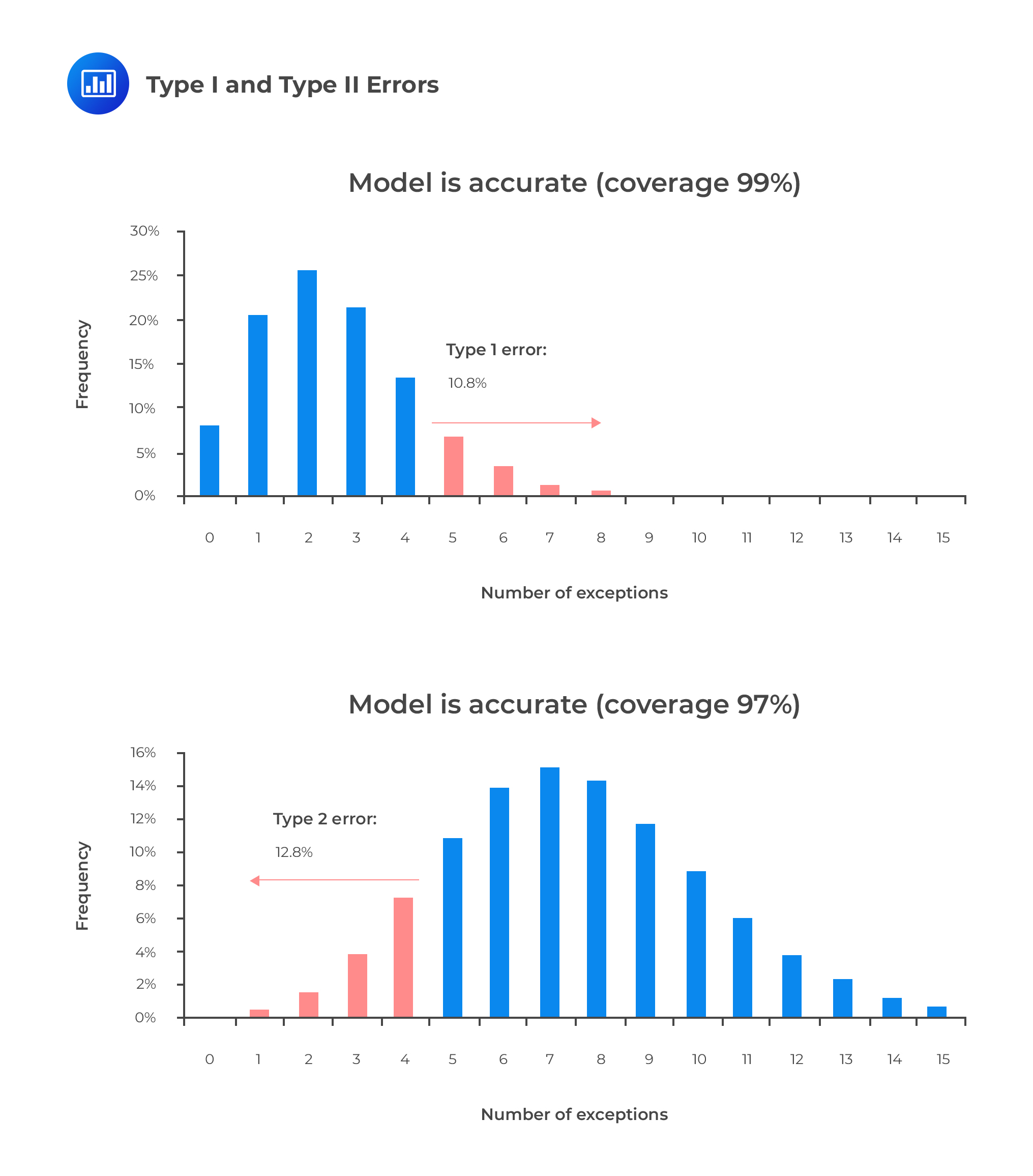
The figures below illustrate the two types of errors. Let’s consider an example where daily VaR is computed at a 99% confidence level for a 250-day horizon. Assuming that the model is correct, the expected number of days when losses exceed VaR estimates is 250 ∗ 0.01 = 2.5. If we set the cut-off level for rejecting a model, for instance, to more than 4 exceptions, the probability of committing a type 1 error is 10.8%.

On the other hand, if the model has an incorrect coverage of 97%, the expected number of exceptions is 250 ∗ 0.03 =7.5.

Unconditional Coverage Models

In the context of backtesting, unconditional coverage implies that we do not pay attention to the independence of exception observations or the timing of when such exceptions occur. To determine whether a model is suitable for risk management, all we’re interested in is the number of exceptions. 

One of the most popular unconditional coverage tests was put forward by Kupiec in 1995. Kupiec proposed a log-likelihood ratio (LR) test that examines how many times a financial institution’s VaR is violated over a given span of time, without any consideration of the distance between exceptions. Using a sample of T observations, Kupiec’s (1995) test statistic takes the form:

$$
LR_{UC}=-2 \ln \left(\frac{(1-p)^{T-N} p^{N}}{\left[1-\left(\frac{N}{T}\right)\right]^{T-N}\left(\frac{N}{T}\right)^{N}}\right)
$$

where:

\(p\) = Probability level.

\(T\) = Sample size.

\(N\) = Number of exceptions.

\(LR_{UC}\) = Test statistic for unconditional coverage (UC).

Kupiek’s test calculates the ratio between the maximum probabilities of a result
under two alternative hypotheses. The numerator defines the maximum probability of the observed result under the null hypothesis, while the denominator defines the maximum probability of the observed result under the alternative hypothesis. The decision is then based on the value of the resulting ratio. The smaller the ratio is, the larger the LR statistic will be. If the test statistic is greater than the critical value of χ² distribution, the null hypothesis is rejected. A common practice is to choose an arbitrarily high level of confidence and use it for all testing, such as 95%. At 95% confidence, the critical value of χ² distribution is 3.84. Such a high degree of confidence means that the model will be rejected only if the evidence against it is fairly strong.

The table below shows the nonrejection regions for the number of failures \(N\) based on the probability level \(p\), confidence level \(c\), and time period \(T\).

$$\begin{array}{l|c|c|c|c} {\textbf{Probability}\\\textbf{Level, p}} & {\textbf{Confidence}\\ \textbf{Level, c}} & \bf{T = }\textbf{252 Days} & \bf{T =} \textbf{510 Days} & \bf{T=} \textbf{1000 Days} \\ \hline 0.01 & 99\% & N < 7 & 1 < N < 11 & 4 < N < 17 \\0.025 & 97.5\% & 2 < N < 12 & 6 < N < 21 & 15 < N < 36 \\ 0.05 & 95\% & 6 < N < 20 & 16 < N < 36 & 37 < N < 65 \\ 0.075 & 92.5\% & 11 < N < 28 & 27 < N < 51 & 59 < N < 92 \\ 0.1 & 90\% & 16 < N < 36 & 38 < N < 65 & 81 < N < 120 \\ \end{array}$$

For instance, with one year of data (T = 252), we would expect to observe

N = pT = 1 * 252 = 3 exceptions. However, the VaR user would not be in a position to reject the null hypothesis as long as N is within the less than 7 (N < 7) confidence interval. Values of N greater than or equal to 7 indicate that the VaR is too low or that the model understates the probability of large losses.

We can also see that increasing the sample size paves way for the rejection of the model more easily. For example, at p = 0.05, the interval for 7 = 252 is [6/252 = 0.024, 20/252 = 0.079]; for 7 = 1000, it is [37/1000 = 0.037, 65/1000 = 0.065]. It’s evident the interval shrinks as the sample size increases.

Conditional Coverage in the Backtesting Framework

Up to this point, we have looked at backtesting based on unconditional coverage, in which the timing of exceptions has not been considered. Unconditional variation falls in line with the “independence” assumption, where we treat the probability of tomorrow’s exception as independent of today’s exception.

In reality, however, there could be time variation in the way the exceptions are observed. Conditional coverage allows us to take account of factors that unconditional coverage ignores. Actual exceptions could cluster or bunch closely in time such that if we take the 95% VaR, for instance, the 13 expected exceptions over a 250-day period could occur within a single month. Bunching of exceptions may be indicative of a change in market correlations or the alteration of trading positions. As such, it is important to have a framework that guides us to determine whether bunching, in a given instance, is purely random or caused by one of these events.

P.F. Christofferson, a scholar, developed a measure of conditional coverage that allows for potential timely variation of data. It is basically an extension of the unconditional coverage test statistic, \(\text {LR}_{\text{UC}}\). In addition to Kupiec’s log-likelihood framework, he extends the test to also include a separate statistic for independent exceptions. Aside from checking the correct rate of coverage, this test checks whether the probability of an exception on any particular day is affected by the previous day’s outcome. The overall log-likelihood test statistic for conditional coverage is computed as:

$$ \text {LR}_{\text{CC}} = \text {LR}_{\text{UC}} + \text {LR}_{\text{ind}} $$

where:

\(LR_{CC}\) = Test statistic for conditional coverage (cc).

\(LR_{UC}\) = Test statistic for unconditional coverage (UC).

\(LR_{ind}\)= Test statistic for independence exceptions (find).

Each individual component is independently distributed as chi-squared, and so is the sum. However, we now have two degrees of freedom since there are two separate LR statistics in the test. If the value of the conditional coverage statistic is lower than the critical value of the χ² distribution, the model passes the test.
For higher values, the model is rejected. 

At a confidence level of 95%, for instance, we would reject the model if \(\text {LR}_{\text{CC}} > 5.99\). We would reject the independence term alone if \(\text {LR}_{\text{ind}}\). If exceptions are found to be serially dependent, what should follow is a reexamination of the model to recognize the correlations in the data.

Basel Rules for Backtesting

In a bid to make banks more observant and adherent to the highest level of risk management, the Basel Committee continually releases guidelines on a range of issues. In line with its mandate, the committee has put in place a framework based on the daily backtesting of VAR.

Current guidelines require banks to record daily exceptions to the 99.0% VaR over the previous year. For 250 observations, the expected number of exceptions is 0.01 * 250 = 2.5.

Basel rules put the number of exceptions into three categories:

• The green zone is defined as having up to four exceptions – an acceptable number. The green zone is effectively a “green light” for a bank to continue using the existing model in risk management. Any bank within this zone does not attract penalties imposed in the form of a multiplicative (“scaling”) factor (k).
• The yellow zone is defined as having between five and nine exceptions. Unlike the green zone, the yellow zone attracts penalties and is effectively a call back to the drawing board to develop a better model. The specific scaling factor to be imposed is left at the discretion of supervisors, and, to a large extent, it depends on the reason for the exceptions.
• The red zone is defined as having 10 or more exceptions. Like the zone before it, it comes with an automatic penalty, where the scaling factor is increased from 3 to 4. The penalty is imposed in a nondiscretionary manner. The red zone requires a bank to undertake an extensive review of its model since it would be extremely unlikely to observe 10 or more exceptions if the model was indeed correct. In some cases, a bank may be forced to abandon the model altogether.

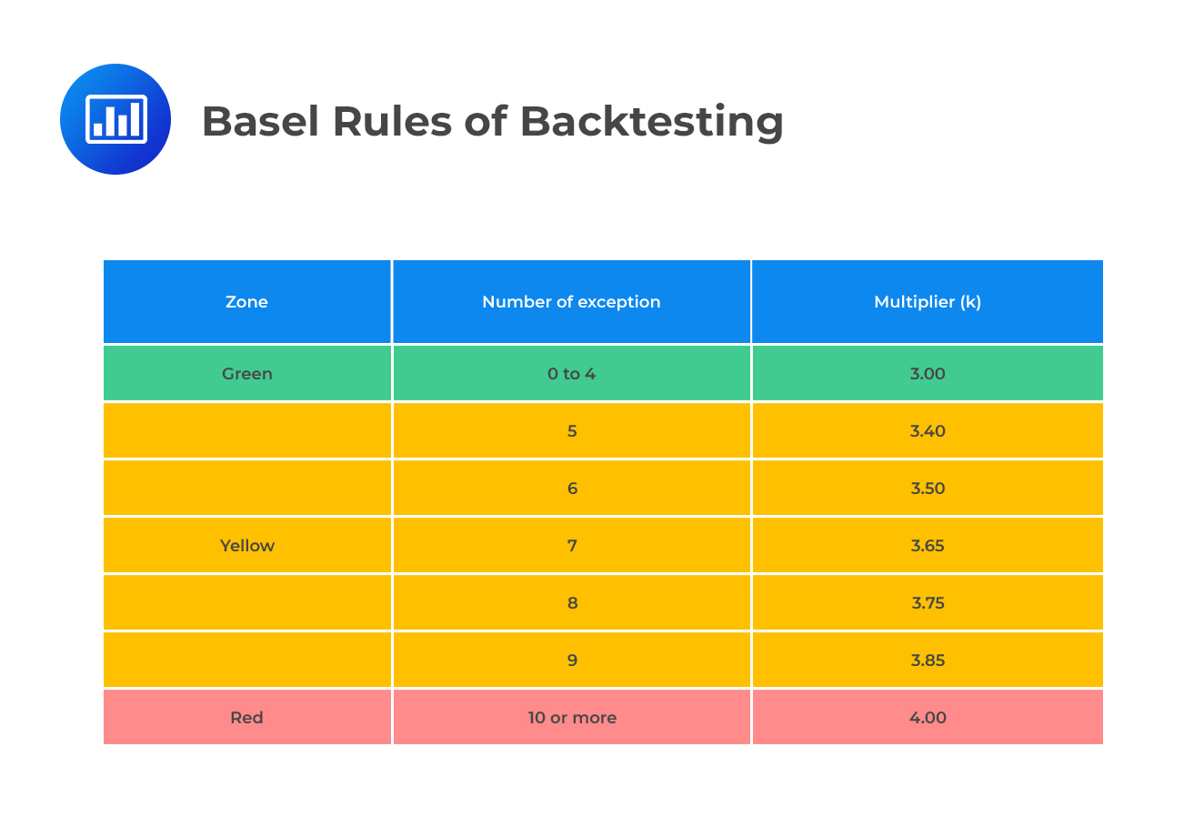As noted earlier, a supervisor enjoys some discretion in the application of penalties for exceptions falling within the yellow zone. The Basel Committee uses these categories:

1. Basic integrity of the model: This implies that a bank’s systems are poor at capturing the risks of the various positions taken. For instance, correlations may have been misspecified. Committee’s guidance: This is a very serious flaw that calls for an increase in the scaling factor penalty that should apply immediate corrective action. For instance, a supervisor may be required to authorize a substantial review of the model and take action to ensure that this occurs.

2. Deficient model accuracy: This implies that the model does not measure the risk exposure of some instruments with enough precision. Committee’s guidance: A lack of model precision is a fairly common flaw that occurs in most risk measurement models. Indeed, no single model is fully immune from some kind of imprecision. If there’s reason to believe that a bank’s model accuracy is significantly wanting when compared to other banks, a supervisor should impose the plus factor and set in motion any other necessary corrective action.

3. Intraday trading: The exceptions occurred due to trading activity that occurred within a 24-hour period. It could be a large (money-losing) trading event that happened between the end of the first day and the end of the second day. Committee’s guidance: If the exception disappears with the hypothetical return, the problem is not in the bank’s VAR model. Nonetheless, a penalty “should be considered.”

4. Bad luck: Either the markets’ movement exceeded the model prediction, or they did not move together as expected. Committee’s guidance: Markets may move in an anticipated fashion from time to time. These types of exceptions “should be expected to occur at least some of the time.”Even among “accurate” models, a 100% market movement prediction rate is nearly impossible. There’s no single VaR model that is immune from bad luck.

Question

Martin, the Chief Risk Officer (CRO) of Zenith Bank, is reviewing the bank’s risk management framework to ensure compliance with the latest Basel regulations, particularly in the domain of backtesting. The bank employs a Value-at-Risk (VaR) model to estimate potential losses on their trading portfolio.

Having experienced a few unexpected losses in the recent past, Martin is keen on understanding the implications of these losses with respect to the Basel requirements for backtesting. 

Given this context, which of the following statements correctly outlines the Basel rules for backtesting?

A. If the number of exceedances is within the acceptable range, the bank should consider revising its VaR model.

B. Exceedances in the VaR model are indicative of the model’s accuracy and can lead to an increase in the capital charge, depending on the number of breaches.

C. Basel regulations focus only on the magnitude of losses and not on the frequency of exceedances.

D. Zenith Bank is required to backtest its VaR model only when unexpected losses occur, according to Basel rules.

Solution

The correct answer is B.

The Basel regulations require banks to regularly backtest their VaR models. If the number of actual losses exceeding the VaR estimate is too high over a certain period (typically a year with 250 observations), it indicates the model may not be accurately capturing the risks. Depending on the number of exceedances or breaches, this can lead to an increased capital charge for the bank.

A is incorrect because while it’s good practice to regularly review and possibly revise the VaR model, the Basel rules don’t dictate a revision solely because the number of exceedances is within an acceptable range. It’s when the exceedances are beyond the acceptable threshold that the capital charge is adjusted, reflecting increased model risk.

C is incorrect because the Basel regulations for backtesting focus on both the magnitude and frequency of exceedances. It’s the number of breaches over a set period that determines the potential adjustment to the capital charge, not just the size of the losses.

D is incorrect because the Basel rules mandate regular backtesting of the VaR model, irrespective of whether unexpected losses occur. While unexpected losses might necessitate an internal review of the model, Basel requires ongoing backtesting as a standard procedure.

Things to Remember

• Basel regulations mandate banks to regularly backtest their Value-at-Risk (VaR) models.
• Exceedances or breaches in VaR models indicate potential inaccuracies in risk estimation.
• An elevated number of breaches over a typical period (like a year) might result in a higher capital charge for a bank.
• The number of actual losses that surpass the VaR estimate, both in magnitude and frequency, are crucial for backtesting.
• Continuous backtesting is a standard procedure required by Basel, not just something conducted after unexpected losses.
• While unexpected losses might signal the need for an internal review, Basel regulations emphasize consistent backtesting and model accuracy.