Credit Value Adjustment (CVA)

After completing this reading, you should be able to:

• Explain the motivation for and the challenges of pricing counterparty risk.
• Describe credit value adjustment (CVA).
• Calculate CVA and CVA as a spread with no wrong-way risk, netting, or collateralization.
• Evaluate the impact of changes in the credit spread and recovery rate assumptions on CVA.
• Explain how netting can be incorporated into the CVA calculation.
• Define and calculate incremental CVA and marginal CVA and explain how to convert CVA into a running spread.
• Explain the impact of incorporating collateralization into the CVA calculation, including the impact of the margin period of risk, thresholds, and initial margins.
• Describe debt value adjustment (DVA) and bilateral CVA (BCVA).
• Calculate DVA, BCVA, and BCVA as a spread.
• Describe wrong-way risk and contrast it with right-way risk.
• Identify examples of wrong-way risk and examples of right-way risk.
• Discuss the impact of collateral on wrong-way risk.
• Identify examples of wrong-way collateral.
• Discuss the impact of wrong-way risk on central counterparties.
• Describe the various wrong-way modeling methods, including hazard rate approaches, structural approaches, parametric approaches, and jump approaches.
• Explain the implications of central clearing on wrong-way risk.

The Motivation for and the Challenges of Pricing Counterparty Risk

Valuation of counterparty risk refers to the practice of attaching a value to the risk of all outstanding positions with a given counterparty. For instance, let’s assume that a trader is planning to engage in an interest rate swap with a double-A counterparty whose outstanding debt is priced at a credit spread of 150 basis points per year. Assume that the notional value of the swap is $500 million.

In these circumstances, the trader will want to ensure that the trader settles for a rate that takes into account counterparty risk, i.e., the possibility that the counterparty will default on contractual payments once the swap is underway. To put a price tag on this risk, the trader will have to consider all of the following:

• Any existing trade the trader already has with the counterparty may increase or even reduce the risk of the new trade (thanks to netting).
• Any collateral agreement the trader could negotiate with the counterparty that may reduce risk
• There may be ways to hedge the default of the counterparty since it has debt trading in the market.

In general, there are two key components needed to price counterparty risk:

• The credit exposure, which is influenced by (I) any existing contracts and (II) risk mitigants such as netting and collateral
• The default probability of the counterparty

Why is pricing Counterparty risk important?

• Correct pricing of counterparty risk helps to ensure that earnings information put out by a firm is accurate.
• Pricing data can be used by trading desks and businesses to decide which trades to pursue and which ones to turn down. A trade is considered viable and economically feasible if its profit is greater than its cost.

When pricing counterparty risk, best practice calls for clear and well-organized responsibilities where the person or office tasked with the calculation process is specified.

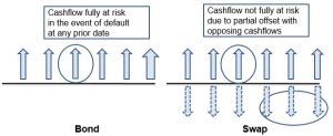
Pricing counterparty risk (derivative contracts), however, is a difficult endeavor, particularly when compared to the pricing of bonds. With bonds, payments are made in only one direction once the investment has been made at the onset of the contract, and a default charge is easily incorporated when discounting scheduled cashflows. With derivatives, contracts are bilateral, with payments often being made in both directions at specified times during the life of the contract. In addition, cash flows may be fixed, floating, or contingent.

The figure below helps to visualize the problem with derivatives. Looking at bonds, a given cashflow is fully at risk (there’s a chance all of it will be lost) in the event of a default. In the swap case, only a fraction of the cashflow will be at risk because there’s an opposing cashflow that offsets the outflow to some degree. Although the risk on the swap is clearly smaller due to this effect, it is hard to determine the fraction of the swap cashflows that are indeed at risk. The amount at risk will depend on many factors, including forward rates and volatilities.

Figure 1 – Bond Cashflows vs. Swap Cashflows

Credit Value Adjustment (CVA)

Credit valuation adjustment, CVA, is a change to the market value of derivative instruments to account for counterparty credit risk. It can also be interpreted as the expected value or price of counterparty risk.

Mathematically, CVA is the difference between the risk-free value and the true portfolio/position value that takes into account the possibility of a counterparty’s default. 

$$\text{Risky value} = \text{risk-free value} – \text{CVA}$$

The equation above implies that it is possible to separate responsibilities in an institution and have a desk responsible for risk-free valuation and another one to determine the risky (counterparty) component. A swap trader, for example, can take on the task of pricing the swap as if it were risk-free and then rely on someone else in the office to determine the counterparty risk charge.

CVA Formula (In the absence of Wrong-way Risk)

Ignoring wrong-way risk implies that we assume independence between default probability, exposure and recovery values. Under such assumptions, the CVA is calculated as follows:

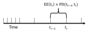
$$\text{CVA}=-\text{LGD}\sum_{i=1}^{m}EE(t_{i})×PD(t_{i-1}, t_{i})$$

Where:

• Loss given default, LGD, is the percentage amount of the exposure expected to be lost in the event the counterparty defaults (Recall that LGD = 1 – recovery rate)
• Expected exposure is the discounted expected exposure for all relevant future dates \(t_{i}\)
• Default probability, PD, is the marginal probability of default between dates \(t_{i-1}\) and \(t_{i}\).

The expected exposure and default probability are computed for each time period \((t_{i-1}, t_{i})\)

Figure 2 – Illustration of CVA formula

The assumption that there’s no wrong-way risk means that the three components as well as discount factors can be calculated by different departments within an institution

Professor’s note: The CVA begins with a negative sign because it is a cost to the counterparty

CVA as a Spread

Instead of calculating the CVA as a stand-alone value, we can also express it as a spread (annual charge). To do so, we divide the CVA by the unit premium of a risky annuity value for the maturity in question. This yields an annual spread expressed in basis points. The spread would effectively be a charge to the weaker counterparty. Assuming that the EE is constant over time and equal to its average value, EPE, CVA as a running spread is computed as follows:

$$\frac{\text{CVA}(t,T)}{CDS_{\text{premium}}(t,T)}=-\text{EPE}×X^{\text{CDS}}$$

Where:

\(CDS_{premium}(t,T)=\text{unit premium value of a CDS (risky annuity)}\)

\(X^{CDS}=\text{CDS premium that corresponds to the maturity date T (credit spread)}\)

The left-hand side of the equation above represents CVA as a running spread.

It is important to emphasize the assumptions we have made so as to estimate CVA as a running spread:

• EPE is constant until maturity
• Probability of default is constant until maturity
• Both the EE and PD are symmetric over the entire profile

Example

An interest rate swap trading desk wishes to come up with a quick estimate of the CVA spread on a swap. As per the department tasked with calculating counterparty exposure, the EPE stands at 6%. A CDS with the counterparty as the reference entity attracts a premium of approximately 200 basis points per year. Determine the CVA as a running spread.

Solution

The CVA as a running spread is computed as follows:

$$\begin{align*}\frac{CVA(t,T)}{CDS_{premium}(t,T)}&=-EPE×X^{CDS}\\&=-6\%×2\%\\&=-0.12\%\\&=-12 \text{basis points}\end{align*}$$

Having determined the CVA as a spread, the trading desk can now estimate approximately the P&L impact of this by pricing the same swap but paying 12 bps more on the pay leg (or receiving 12 bps less on the receive leg). The other option would be to add/subtract a CVA charge of 12 basis points to one leg of the trade.

The impact of Changes in the Credit Spread and Recovery Rate Assumptions on CVA

CVA is impacted by each of the following:

• Credit spread levels
• Overall shape of the credit curve
• Recovery rate
• Basis risk arising from LGD assumptions

Impact of Credit Spread

Generally, as the credit spread of the counterparty increases, the CVA increases (becomes less negative). However, the impact is not linear because default probabilities are limited to 100%. If the counterparty is very close to default, the CVA tends to decrease (become more negative)

In default, the CVA falls to zero

Figure 3 – CVA as a function of the credit spread of the counterparty (Forward contract-type exposure)

$$\small{\begin{array}{|l|l|}\hline\textbf{Spread (bps)} & \textbf{CVA}\\ \hline150 & -1,074\\ \hline30 & -1,999\\ \hline600 & -3,471\\ \hline1,200 & -5,308\\ \hline2,400 & -6,506\\ \hline4,800 & -6,108\\ \hline9,600 & -4,873\\ \hline\text{Default} & 0\\ \hline\end{array}}$$

Credit: The xVA Challenge Counterparty Credit Risk, Funding, Collateral, and Capital by Jon Gregory

Shape of the Credit Spread Curve

• With an upward sloping curve, defaults are back loaded.
• With a downward sloping curve, defaults are front loaded
• With a flat curve, defaults are evenly spaced until maturity

As a result, the CVA will be lower (more negative) for an upward-sloping curve compared to a flat and a downward sloping curve. It is highest (least negative) with a downward sloping curve

Recovery Rate

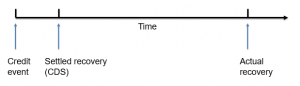
An increase in the recovery rate increases the implied probability of default but reduces the CVA. A related point has much to do with recovery timing: Whereas CDSs are settled quickly following a default event either by way of a CDS auction cash settlement mechanism or the sale of the debt security in the market, bilateral OTC derivatives take time to settle. That’s because the underlying transactions such as netting (less collateral) are often quite difficult to define given a large number of trades.

This gives rise to two types of recovery: settled and actual recovery

• Settled recovery refers to the recovery that could be achieved following the credit event by trading out of a claim say, by selling a defaulted bond.
• Actual recovery is the recovery paid on a derivative at the conclusion of a bankruptcy or similar process

 Figure 4 – Illustration of Settled Recovery and Actual Recovery

Example

• A 20% recovery assumption for both settled and actual recovery rates will produce a lower (more negative) CVA compared to a 40% recovery assumption.
• However, a 10% settled recovery rate and a higher 40% actual recovered rate gives a much higher (less negative) CVA

Figure 4 – CVA of the base case IRS for different recovery assumptions

$$\small{\begin{array}{|l|l|}\hline\textbf{Recovery (Settled/final)}&\textbf{CVA}\\ \hline\text{20% both}&-2,072\\ \hline\text{40% both}&-1,999\\ \hline\text{60% both}&-1,862\\ \hline\text{10%/40%}&-1,398\\ \hline\end{array}}$$

Incorporating Netting into CVA Calculations

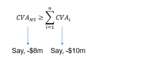
As a risk mitigant, netting reduces CVA. A group of n transactions with the same counterparty under one netting agreement is called a netting set (NS). The CVA for a given netting set must be greater than or equal to the sum of stand-alone CVAs:

Figure 5 – Illustrating the impact of Netting on CVA

Thus, one must evaluate the change in CVA before a trade has been executed

A new trade should be priced so that its profit at least offsets any increase in CVA.

Mathematically,

$$\text{CVA}_{i}^{incremental}=\text{CVA}_{NS+i}-\text{CVA}_{NS}$$

The ability to calculate the incremental CVA helps the trading desk to attach a risk charge to every new trade brought in by a trader or sales person. That way, it is possible to come up with a compensation mechanism that is commensurate with the risk of the new trade

The Impact of Incorporating Collateralization into the CVA Calculation

Collateral reduces CVA (results in a less negative CVA value) but it only changes the counterparty’s expected exposure, EE, not its PD

Minimum transfer amounts increase CVA (result in more negative CVA value since they increase exposure linearly.

Incremental CVA

As noted earlier, Incremental CVA is the change (or increment) in CVA that a new trade will create, taking netting into account.

It is derived as follows:

$$\text{CVA}^{incremental}_{i}=-LGD\sum_{i=1}^{m}EE_{i}^{incremental}(t_{i})×PD(t_{i-1},t_{i})$$

If you look closer, the incremental CVA looks pretty much like the original CVA. The only difference is that the original stand-alone EE is replaced by the incremental EE:

$$\text{CVA}=-LGD\sum_{i=1}^{m}EE(t_{i})×PD(t_{i-1}, t_{i})$$

The incremental EE is the change in EE at each point in time caused by the new trade, which impacts the original exposure

Incremental CVA Example

The table below gives the incremental CVA calculations for a seven-year USD swap paying fixed with respect to four different existing transactions and compared to the stand-alone value. We assume that the credit curve is flat at 300 bps with a 60% LGD.

Figure 6 – the incremental CVA calculations for a seven-year USD swap

$$\small{\begin{array}{|l|c|}\hline\textbf{Existing transaction}& \textbf{Incremental CVA}\\ \hline\text{None (stand-alone)} & -0.4838\\ \hline\text{Payer IRS USD 5Y} & -0.4821\\ \hline\text{Payer swaption USD 5*5Y} & -0.4628\\ \hline\text{xCCY USDJPY 5Y} & -0.2532\\ \hline\text{Receiver 1RS USD 5Y} & -0.1683\\ \hline\end{array}}$$

Observations

• The incremental CVA can never be lower (more negative) than the stand-alone CVA
• The incremental CVA is only slightly reduced for a very similar existing trade (5-year IRS payer). This indicates a high positive correlation between the two trades.

Marginal CVA

Marginal CVA enables the trading desk to break down netted trades into trade level contributions that sum to the total CVA. As an ex-post measure, it is determined after the portfolio CVA has been calculated and then allocated to trades

In other words, the marginal CVA is found by breaking down the CVA for any number of transactions into transaction-level contributions that sum to the total CVA. The breakdown is carried out based on certain criteria

The marginal CVA helps the trading desk to single out transactions that have the greatest impact on a counterparty’s CVA. The incremental CVA and marginal CVA can be the same, depending on the allocation criteria.

Debt Value Adjustment

Up to this point, we have assumed that the party calculating the CVA (party with positive exposure) has a zero chance of default. In a transaction involving a counterparty and a large multinational financial institution, for example, such an assumption would appear fairly innocuous. Indeed, it falls in line with the “going-concern” accounting principle, where every transaction that appears on the financial statements is initiated upon the assumption that the business will remain in existence (solvent) for an indefinite period. That means the financial institution is assumed to have zero counterparty risk from the perspective of the counterparty. However, the events of the 2007/09 financial crisis deconstructed and poked big holes in this assumption, seeing that several large institutions previously considered financially invincible and too big to fail went down.

As a result, international accountancy practices now recognize that all trades have bilateral counterparty risk. They allow large institutions to consider their own default in the valuation of their liabilities. Which brings us to debt value adjustment.

Debt value adjustment, DVA, is the counterparty risk of the institution writing the contract. It can be thought of as the negative of CVA. In other words, an institution’s DVA is the counterparty’s CVA. DVA is actually a benefit to the defaulting institution. That’s because if the institution happens to default when its MTM exposure is negative, the institution will only pay the counterparty the recovery amount, which is just a fraction of what they owe. The difference between the amount recovered by the counterparty and the actual amount the institution owes is a gain to the institution.

While CVA considers only positive exposure, the DVA considers only negative exposure.

Bilateral CVA

Bilateral CVA is CVA that incorporates an entity’s own credit risk into the derivative valuation process. It is built upon the recognition that the creditworthiness of both parties in a bilateral contract matter. In a transaction between a small counterparty and a larger financial institution, an informed counterparty (viewed as the “underdog”) would be expected to adjust for the institution’s credit risk when valuing the transaction.

$$\text{BVCA}=\text{CVA}+\text{DVA}$$

$$\text{CVA}=-LGD_{C}\sum_{i=1}^{m}EE(t_{i})×PD_{c}(t_{i-1},t_{i})×(1-PD)_{p}(0, t_{i-1})$$

$$\text{DVA}=-LGD_{P}\sum_{i=1}^{m}EE(t_{i})×PD_{p}(t_{i-1},t_{i})×(1-PD)_{c}(0, t_{i-1})$$

Where;

NEE = negative expected exposure (EE from the counterparty’s perspective)

P and C indicate the party making the calculation and their counterparty, respectively.

BCVA as a Spread

We can rewrite BCVA in terms of the EPE and ENE as follows:

$$\text{BCVA}=-\text{EPE}×\text{Spread}_{C}-\text{ENE}×\text{Spread}_{P}$$

If we assume that   is the opposite of, then

$$\text{BCVA}≈-\text{EPE}×(\text{Spread}_{C}-\text{Spread}_{p}).$$

Example:

An interest rate swap trading desk wishes to come up with a quick estimate of the CVA spread on a swap

Given: EPE\(=6%\); ENE\(=-4\%\); \(\text{spread}_{c}=200 bps\); \(\text{spread}_{p}=100 bps\)

From the perspective of the trading desk, 

\(\text{BCVA}=-6\%×2\%-(-4\%×1\%)=-0.08\%=-8 bps\)

Hence, the trading desk will charge the counterparty 8 bps for the overall counterparty risk.

Compared with the previous example, we can see that the BCVA is reduced from the (unilateral) CVA calculation of 12 bps

Wrong-way Risk vs. Right-way Risk

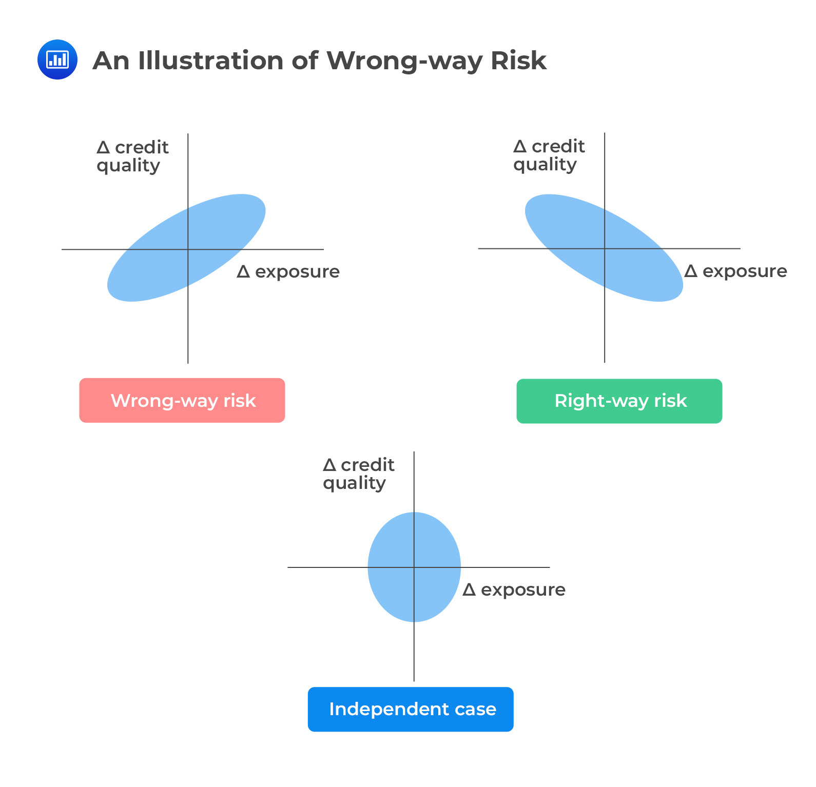
One of the key issues that arise when analyzing CCR is a wrong-way risk, defined as the risk that occurs when exposure to a counterparty is adversely correlated with the credit quality of that counterparty. In short, it is the risk that default risk and credit exposure will show an unfavorable dependence and tend to increase together. It is important to note that wrong-way risk does not arise with fixed-rate loans.

Wrong-way risk increases counterparty credit risk and therefore increases CVA. At the same time, it leads to a reduction in DVA.

Right-way risk, on the other hand, exists when there’s a favorable dependence between exposure and credit quality.  In this case, the linkage between exposure and the counterparty’s probability of default produces an overall decrease in counterparty risk. That implies CVA decreases, but at the same time, DVA increases.

Both wrong-way and right-way risks are frequently observed in practice. For instance, consider the case of a middle-level bank that holds a large unhedged portfolio of derivatives with a dealer. If market variables move in such a way that the value of the derivatives to the bank is negative, the bank will be losing money. If losses accumulate for the bank, it is likely that the bank will be unable to make the required payments and default. While that happens, the value of the portfolio to the dealer will be positive, and therefore the dealer’s exposure will be increasing. This results in a wrong-way risk for the dealer. The probability that the bank will default when it has a large negative exposure is large. 

From a historical perspective, wrong-way risk has commanded more attention than right-way risk, but both types of risk are hugely important, and it is imperative that institutions strive to increase right-way risk while decreasing wrong-way risk.

Figure 1 – An Illustration of Wrong-way Risk

Examples of Wrong-way Risk

Put Option

If a trader buys a put option on a stock whose performance has a strong positive correlation with the counterparty’s performance, there’s an obvious case of wrong-way risk.

Consider a situation where Smart Tech buys a three-month put option from Cortana Inc., with Alpha stock as the underlying. At expiry, Alpha stock has a price of $45, and the put is, therefore, ITM with a value of $5 (ignoring the premium). During the same period, Cortana’s stock has plummeted after a landmark lawsuit loss against another firm. In this case, the credit exposure of Smart Tech to Cortana Inc. has increased, but this has coincided with a deterioration in Cortana’s creditworthiness

This situation can also be brought about by macroeconomic factors such as interest rates and inflation, which could cause a fall in the underlying asset (Alpha stock) while also introducing financial instability of the counterparty (Cortana)

Foreign currency Transactions

Consider a case where a commercial bank in a developing market such as Venezuela enters into a cross-currency swap with a U.S. bank (developed market). Under the terms of the deal, the commercial bank (the counterparty) will deliver developed market currency (USD) in return for local currency. If macroeconomic conditions take a turn for the worse such that the local currency declines (depreciates), the transaction value to the U.S. bank substantially increases; the exposure increases significantly. The counterparty will be required to spend more of the local currency to deliver U.S. dollars as agreed; the risk of default, therefore, increases.

An increase in exposure for the U.S. bank coupled with an increase in the risk in the counterparty’s risk of default amounts to wrong-way risk. But if the U. S. bank’s exposure increases but the counterparty’s probability of default declines, there will be a reduction in counterparty risk. That would effectively be a case of right-way risk

Total Return Swap

Consider a case where Metropolitan Bank, based in the Philippines, enters into a total return swap (TRS) with Alpha Inc. As per the swap agreement, Metropolitan pays the total return on its bond (BND_MTN_AA) and receives a floating rate of LIBOR plus 5% from Alpha Inc. If interest rates start rising globally, the credit position of Alpha Inc. will start deteriorating, and this will coincide with an increase in its payment liabilities to Metropolitan

Credit Default Swap

Consider a different case where Metropolitan Bank enters into a credit default swap with Alpha Inc. as the protection seller. The reference asset is a $50m bond investment in Bank ABC. Thus, Alpha Inc. provides credit protection to Metropolitan in the event Bank ABC defaults on its obligations. If macroeconomic conditions take a turn for the worse, there’s a real chance that Bank ABC will default, and at the same time, the protection seller (Alpha Inc.) will be unable to fulfill its obligations.

Commodity Forward

A commodity entered with a consumer who seeks to hedge the price of a good can yield wrong-way risk.

Consider the case of an airline wary of an increase in the oil market. The airline decides to use derivatives to hedge all of its consumption by entering into a forward contract. As per the contracts, the dealer agrees to sell oil in the future at $30 per barrel. As maturity approaches, the price rises to $50 per barrel. This is a win for the airline because they will now be buying cheap. But that also means there’s a big loss for the dealer. The problem gets worse if the dealer has concentrated (many) short positions because there will be a flood of claims tabled by various parties (possibly other airlines). This will put intense pressure on the credit quality of the dealer

In this case, the positive value (exposure) from the perspective of the airline coincides with an increase in the dealer’s probability of default. This increases overall counterparty risk and produces wrong-way risk.

Examples of Right-way Risk

Commodity Forwards may also yield right-way risk when entered into with a producer who seeks to hedge the price of their goods.

Consider the case of an oil producer wary of a decline in the oil market. The producer decides to use derivatives to hedge 50% of their production by entering into a forward contract. As per the contracts, the dealer agrees to buy oil in the future at $50 per barrel. As maturity approaches, the price declines to $30 per barrel. In this case, the producer (the counterparty) is likely to default, and they are losing money on the unhedged part of their production. But with the price of oil so low, the value of the forward contracts to the dealer is also low. In this case, the derivatives have a positive value (exposure) to the oil producer and a negative value to the derivatives dealer. 

As such, the dealer’s exposure is likely to be low when the oil producer (counterparty) defaults.

Call Option

Consider a situation where Smart Tech buys a three-month call option from Cortana Inc., with Alpha stock as the underlying.

Strike price: $50; Type: European; Expiry: Day 90; Underlying: Alpha Stock

At expiry, Alpha stock has a price of $55, and the call is, therefore, ITM with a value of $5 (ignoring the premium). During the same period, Cortana’s stock rallied after a landmark lawsuit wins against another firm.

In this case, the credit exposure of Smart Tech to Cortana Inc. has increased, but this has coincided with an improvement in Cortana’s creditworthiness.

General vs. Specific Wrong-way Risk

• Specific wrong-way risk(SWWR) arises due to the specific characteristics of the counterparty or the transaction,
  • That includes things like a rating downgrade, poor earnings, or litigation.
• General wrong-way risk(GWWR)—also known as conjectural wrong-way risk, is driven by macro-economic relationships 
  • That includes things like interest rates, pandemics, political unrest, or inflation in a particular region.
• The two types of risk differ as follows:

Figure 2-General WWR vs. Specific WWR

$$ \small{\begin{array}{c|c} {\textbf{GWWR}} &\textbf{SWWR} \\ \hline \text{Should be priced and managed correctly} &{\text{Should in general be avoided, as it may} \\ \text{be extreme}} \\ \hline {\text{Relationships may be detectable using} \\ \text{historical data}} &{\text{Hard to detect except by a knowledge of} \\ \text{the relevant market, counterparty and the} \\ \text{economic rationale behind transaction}} \\ \hline {\text{Can potentially be incorporated into} \\ \text{pricing models}} &{\text{Difficult to model and risky to use naïve}\\ \text{correlation assumptions; should be addressed} \\ \text{qualitatively via methods such as stress-testing} }\\ \end{array} }$$

Challenges Associated with Quantifying Wrong-way Risk

To quantify WWR, the risk manager has to model the relationship between credit, collateral, funding, and exposure.

The modeling process is complex due to a number of issues:

Uninformative historical data

Although historical data may contain some information on WWR, extracting the underlying relationships is challenging. Time series analysis or correlation may not help

Misspecification of relationship

Correlation can be zero, but it does not imply independence! Rather than exhibiting a correlation, the relationship between two events may be a cause-and-effect type of relationship.

Direction

The direction of WWR is not always clear. For example, low-interest rates usually indicate a recession and tough credit conditions, but high-interest rates could well trigger the same conditions

The Impact of Collateral on Wrong-way Risk

Collateral is a good way to reduce exposure. WWR can cause the exposure to increase significantly, and therefore it is important to consider the impact of collateral on WWR.

• When the exposure is increasing gradually, collateral does a good job of minimizing the impact of wrong-way risk because derivative agreements have clauses that require parties to post collateral after a certain threshold is exceeded. This extra collateral is therefore easy to request and receive.
• But in cases where there’s a sudden jump in exposure, collateral does very little in the way of mitigating WWR
  • For example, if there happens to be a 20% currency devaluation that coincides with sovereign default, collateral is rendered almost useless because it may not be received at all

The impact of wrong-way risk on central counterparties

CCPs may be particularly prone to WWR because they rely so much on collateral as protection. CCPs tend to closely manage and monitor membership by only admitting parties with a certain credit quality

Moreover, all members have to provide an initial margin and also make contributions to the default fund that serves as an extra layer of cushion. But there’s a problem: These initial margins and default fund contributions are based on the portfolio’s market risk. As such, this separation of credit risk and market risk may culminate in a situation where collateral requirements ignore WWR!

For CDS in particular, CCPs are faced with an uphill task trying to quantify the WWR component when setting initial margins and default fund contributions. That’s because higher credit quality can increase WWR (when things take a turn for the worse, previously highly rated credits can get hit quite hard!).

The collateral posted carry WWR; members may post highly risky or illiquid securities.

Wrong-Way Collateral

Wrong-way collateral occurs when an increase in exposure to a counterparty is accompanied by a decrease in the value of the collateral. In other words, it arises when the exposure to a counterparty is adversely (negatively) correlated with the value of collateral posted by that counterparty.

Ideally, collateral should reduce wrong-way risk by ensuring that if the counterparty defaults, there’s a “fallback” asset that can be seized to offset at least part of the loss.  But there’s trouble if an increase in exposure coincides with a decrease in the value of collateral. In such circumstances, the collateral may still offer a certain level of protection against loss, but this may be much lower than initially envisioned.

Examples of Wrong-way Collateral

Payer interest rate swap collateralized by a government bond

Assume a bank has entered into an interest rate swap as the payer, i.e., the party paying the fixed interest rate throughout the life of the swap. Assume further that the counterparty has offered a high-quality government bond as collateral.

Now remember that bonds and interest rates have an inverse relationship: when the interest rate rises, bond prices fall, and vice versa. So, if interest rates rise, it means the bank will be gaining (winning), and its exposure to the counterparty will increase. However, the value of collateral will decline. This would present a classic case of wrong-way collateral.

Cross-currency swap collateralized by cash in one of the two underlying currencies

Assume an American bank has entered into a cross-currency swap with a Brazilian company. The bank will pay interest denominated in Brazilian reals (BRL) and receive in USD. Further, assume that the Brazilian company has offered collateral in Brazilian reals. In the scenario of a sovereign default in Brazil, the local currency (BRL) will be devalued. This will cause the bank’s exposure to spike and reduce the value of collateral at the same time.

Wrong way-risk modeling approaches

Hazard rate approaches

This approach views the credit spread as a stochastic process and then goes ahead to establish the correlation between the credit spread (“hazard rate”) and the other variables used to model exposure.

This approach can be implemented relatively tractably, as credit spread paths can be generated first, and exposure paths only have to be simulated in cases where a default is observed. The required correlation parameters are observed directly via historical time series of credit spreads and other relevant market variables.

On the downside, simple hazard rate approaches generate only very weak dependency between exposure and defaults. In other words, these approaches generate very weak wrong-way effects.

As an example, a simple hazard rate approach can be approached to model wrong-way risk in an interest rate swap. Credit spreads are modeled through a lognormal process and then correlated to interest rates. For the fixed rate payer, a positive correlation with credit spreads implies higher interest rates in default scenarios, leading to a higher positive exposure and higher wrong-way risk. For a negative correlation, the negative exposure increases (right-way risk).

Figure 2- Interest rate simulations conditional on counterparty default (at some point in the five-year period) for the hazard rate model.

 Figure 2 above shows paths of interest rates generated given defaults incase correlation is negative. This is due to the fact that defaults occur where credit spread are wider and interest rates are lower (implying the negative correlation).

Figure 3: Future values for a receiver interest rate swap conditional on counterparty default for a hazard rate approach with negative correlation.

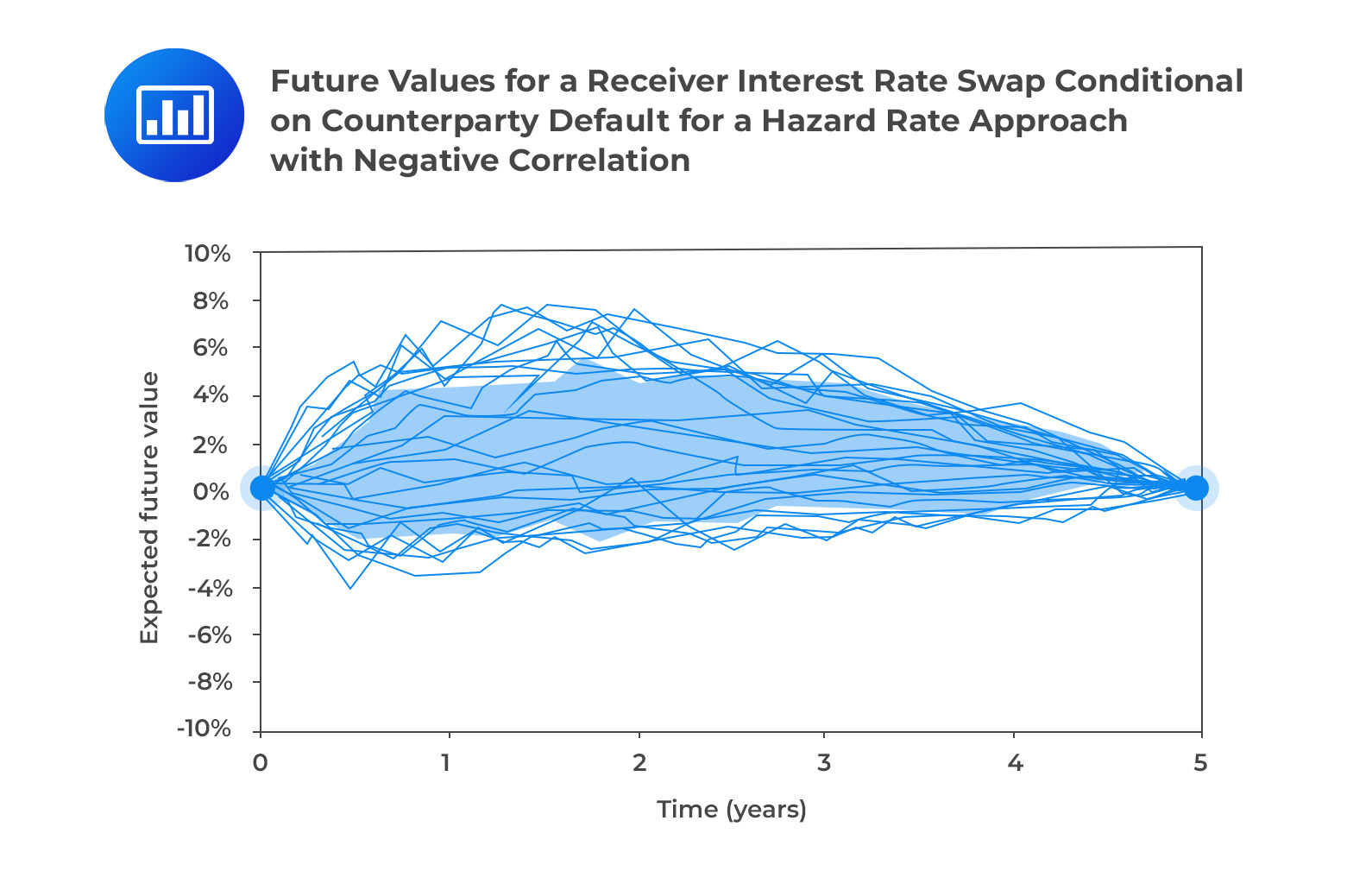From figure 3 above, we can see that swap values are more in -the-money in case of default. This is an impact of WWR thus leading to a higher CVA when the correlation is negative and vise-versa.

Drawback of the approach

This approach generates only weak dependency between exposure and default. The WWR effects are still not strong even when a strong correlation is used.

Structural Approaches

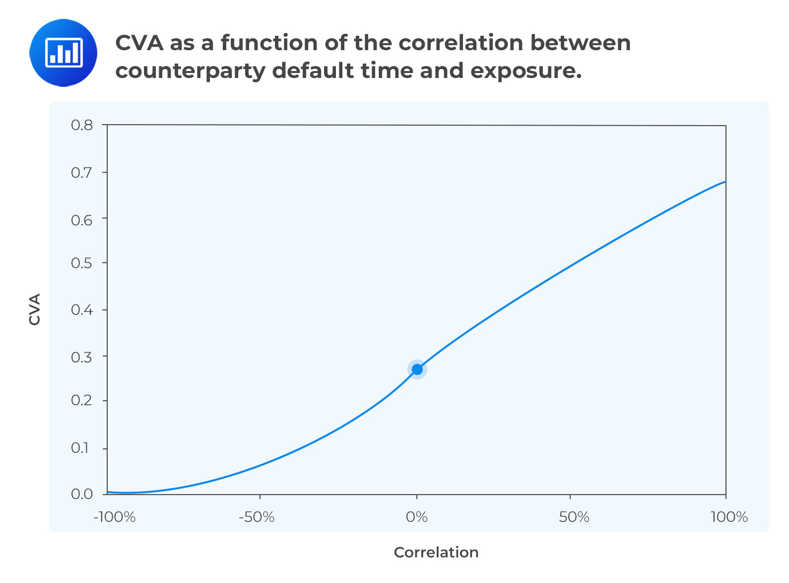
This is a more-simple approach which requires that the dependency between the counterparty default time and exposure distribution be specified.

 Exposure and default distribution are mapped separately into a bivariate distribution. In case of a WWR, positive dependency will lead to an early default time being coupled with a higher exposure. The reverse is true for the right- way-risk.

The advantage of this approach is that the original unconditional values are sampled directly and hence there is no need to recalculate the exposures. The exposure distributions computed initially are used and WWR is added on top of the existing methodology.

When plotted against correlation, it can be seen that CVA is reduced(increased) by negative(positive) correlation due to the effects right way risk (WWR) The effect is stronger and the CVA doubles when correlation is about 0.50. See Figure 4 below.

Figure 4: CVA as a function of the correlation between counterparty default time and exposure. The point marked shows the standard CVA (0% correlation).

Drawbacks of the approach

• Calibrating the correlation being talked about, is difficult since the correlation is not clear.
• It is not appropriate to assume that all the required information for defining the WWR is contained in the original unconditional exposure distribution.

Parametric Approaches

This is a more direct approach that involves parametrically linking default probability to the exposure by simple functions as proposed by Hull and White (2011). An intuitive calibration based on what-if scenario or using historical data to calibrate the relationship may be applied.

When calibration is achieved through historical data, portfolio value for dates in the past need to be calculated and then the relationship between this and the counterparty’s credit spread is examined. If the portfolio is found to have high values with credit spread that exceed the average, is a clear indication of the WWR. The historical data needs to show a meaningful relationship. Furthermore, the current portfolio of trades with the counterparty needs to be of the same nature to that of used in the historical calibration.

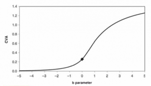
In the Hull and White WWR model, the single parameter (b) drives the relationship, which has an impact similar to the correlation in the structural model.

From figure 5 below, it can be seen that, a positive value will result into a WWR accompanied by a higher CVA. The reverse is true for a negative value.

Figure 5: CVA as a function of the dependency parameter in the Hull and White approach.

Jump approaches

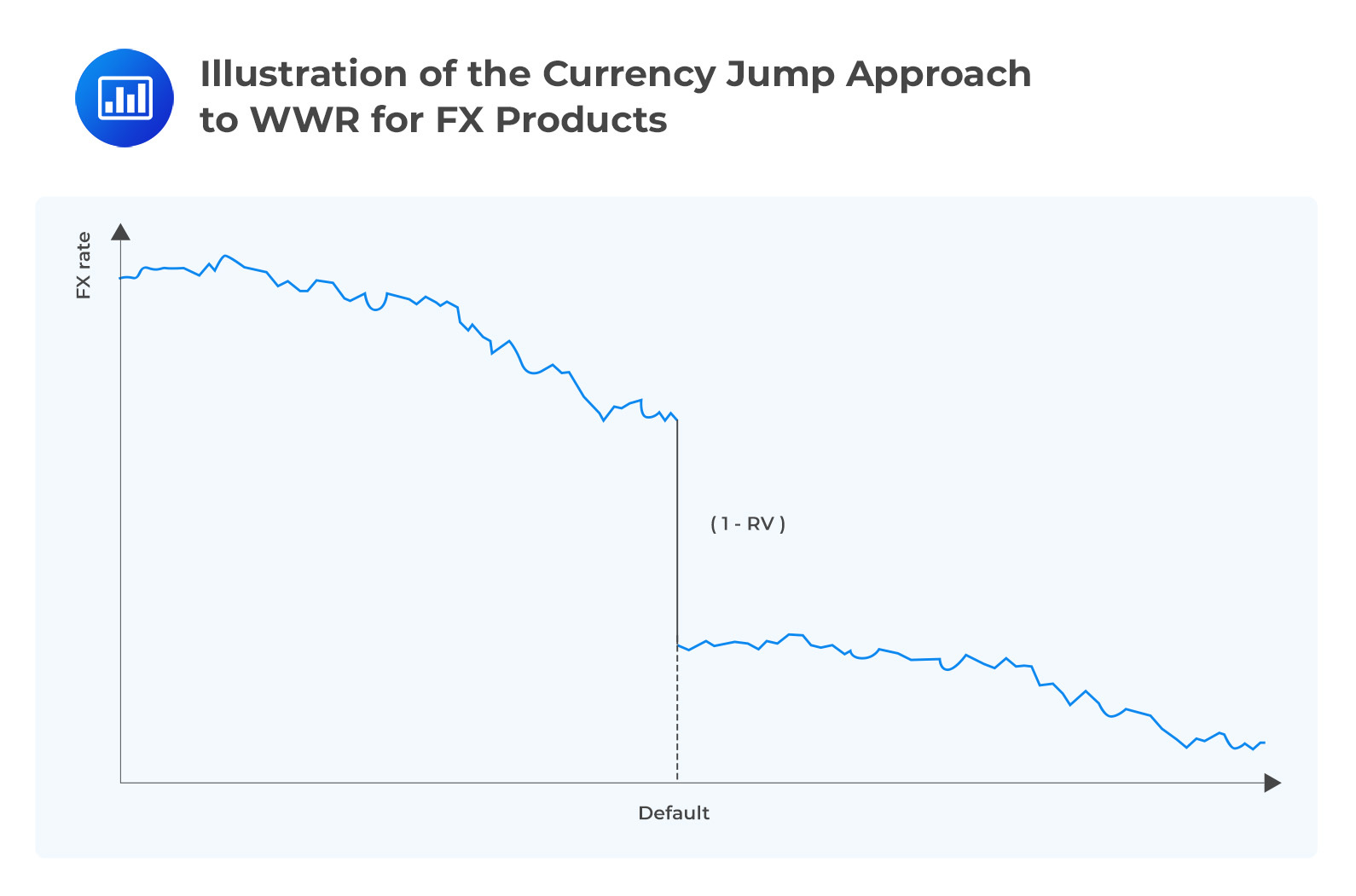
These approaches can apply best in cases where we have specific WWR. The best example here is the FX case. Ehlers and Schonbucher (2006) have paid keen interest on the effect of default on FX rates and considered cases where the hazard rate approach is not suitable to explain empirical data. This is an indication that there is an additional jump in the FX rate at default.

The model proposed by Levy and Levin (1999), to model FX exposures with WWR assumes relevant counterparty FX rate jumps at the counterparty default time.

The jump factor is commonly known as the residual value (RV) factor of the currency and it is assumed that currency depreciates by an amount (1-RV) at the default time of the counterparty and appropriate FX rate jumps.

Figure 6: Illustration of the currency jump approach to WWR for FX products.

Based on historical default data on sovereigns, Levy and Levin showed that sovereigns with better ratings have a larger implied jump. This is probably because their default requires a more severe financial shock, and therefore, the conditional FX rate needs to be increased. The same approach may also be applied to other counterparties. For instance, when a large corporate defaults, we expect it to greatly affect the domestic currency.

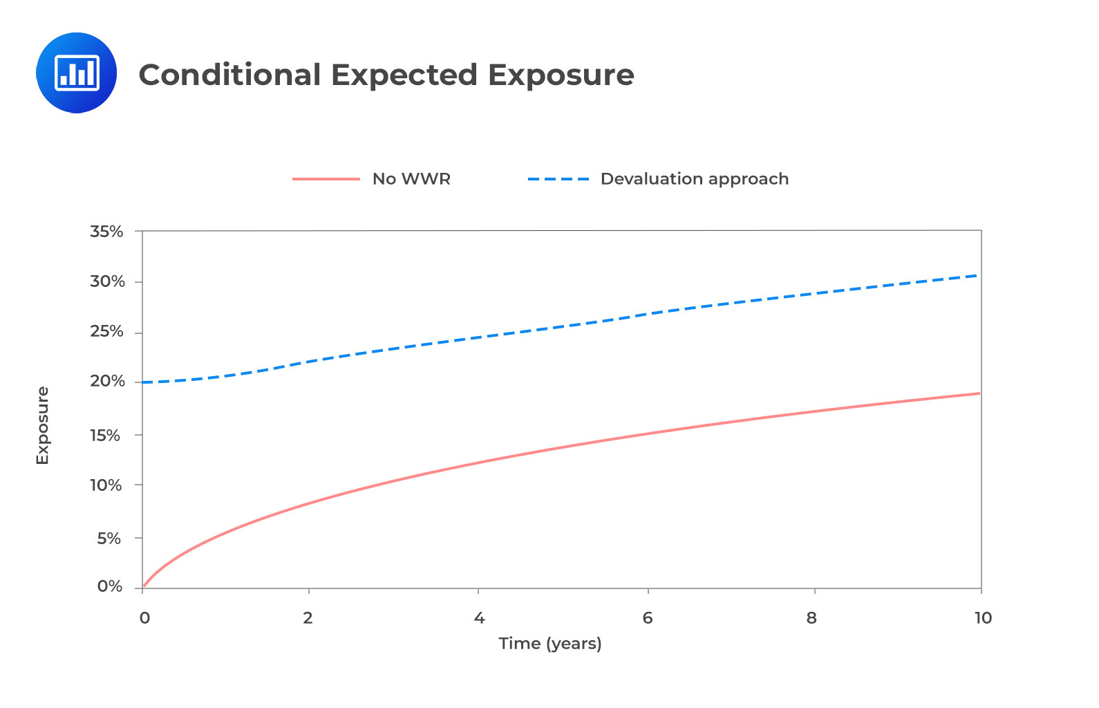
The effect of the conditional expected exposure for the devaluation WWR approach is fairly uniform contrary to the previous conclusions that the impacts of WWR vary greatly with time horizon. It can be assumed that in the short-term, immediate sovereign default may result in a large currency jump (a small RV), while a later default may result in a smaller currency jump (larger RV in the medium/long term.)

Figure 7: Illustration of the conditional expected exposure for the devaluation WWR approach for an FX forward assuming a residual value factor RV = 80%. The FX volatility is assumed to be 15%.

The devaluation approach also applies in CDS markets. Largely, CDS are quoted in US dollars, with a small percentage quoted in other currencies.

Consider table 2 below,

Table 2: CDS Quotes (Mid-Market) on Italy in Both US Dollars and Euros from April 2011

$$\small{\begin{array}{|c|c|c|}\hline\textbf{Maturity} & \textbf{USD} & \textbf{EUR} \\ \hline\text{1Y} & 50 & 35\\ \hline\text{2Y} & 73 & 57\\ \hline\text{3Y} & 96 & 63 \\ \hline\text{4Y} & 118 & 78\\ \hline\text{5Y} & 131 & 91\\ \hline\text{7Y} & 137 & 97\\ \hline\text{10Y} & 146 & 103\\ \hline\end{array}}$$

The only difference between CDS contracts is the currency of cash payment on default. Euro-denominated have a large “quanto” effect and as such, CDS are cheaper by about 30% for all maturities. This matches a RV of about 69% in the event that Italy defaults using five-year quotes (91/131). The RV is time-homogeneous which is in line with the approach discussed above.

Central Clearing and Wrong-Way Risk

Central Counterparties (CCPs) especially those that clear CDS products, are prone to WWR since they rely on collateral as their protection. The common feature of a CCP is that the defaulter pays. i.e., Losses resulting from a clearing member shall be included in the resources dedicated by that clearing member to compensate for the resulting losses. When such losses are imposed on members, the CCP puts itself at the risk of becoming insolvent.

CCPs tend to not associate credit quality and exposure. In order to be a clearing member, the CCP requires that parties must have a certain credit quality and not external credit ratings. However, initial margins and default fund contributions will then be charged, driven primarily by the market risk of their own portfolio. As a result, these CCPs are at risk of implicitly ignoring the WWR.

The problem associated with WWR transactions such as CDS and CCPs is that it is difficult to quantify the WWR component in defining initial margins and default funds. In addition, WWR increases proportionally with increasing credit quality.

It has also been argued that large dealers represent more WWR than smaller credit quality counterparties. As such, it is clear that CCPs require greater initial margins and default fund contributions from better credit quality members.

Question

Alpha Investments, a prominent hedge fund, has been diversifying its portfolio in recent months. Among its new trades, it has entered into a credit default swap (CDS) agreement with Zeta Corp., where Alpha Investments buys protection on a bond issued by Omega Corp., a company in the oil industry. At the same time, Alpha has a separate collateral agreement with Zeta Corp. which is correlated with oil prices. Jenna, the senior risk analyst at Alpha, is evaluating the potential risks associated with this setup.

Based on the given scenario, which statement best describes the type of risk that Alpha Investments is exposed to with respect to its arrangements with Zeta Corp.?

A. Alpha Investments is exposed to right-way risk because as the probability of Omega Corp. defaulting rises, the value of the CDS protection also rises.

B. Alpha Investments is exposed to wrong-way risk due to the correlation between Zeta Corp’s collateral value and Omega Corp.’s creditworthiness.

C. Alpha Investments faces neither wrong-way nor right-way risk as both the CDS and the collateral agreement have mutually exclusive risk factors.

D. Alpha Investments is exposed to right-way risk because an adverse movement in oil prices will improve the value of the collateral with Zeta Corp.

Solution

The correct answer is B.

Wrong-way risk arises when the exposure to counterparty risk increases as the credit quality of the counterparty deteriorates. In this scenario, if oil prices drop (thus affecting Omega Corp.’s creditworthiness), the value of Zeta Corp.’s collateral (which is correlated with oil prices) may also decrease, exacerbating the counterparty risk for Alpha Investments.

A is incorrect because, while it correctly describes right-way risk in general terms, the question focuses on the risks arising from the arrangement with Zeta Corp., not the inherent nature of a CDS.

C is incorrect because Alpha Investments does face wrong-way risk due to the correlation between Zeta Corp.’s collateral value and Omega Corp.’s creditworthiness, as described in the correct answer.

D is incorrect as it inaccurately portrays right-way risk. Right-way risk would mean that an adverse movement in a risk factor would improve the counterparty’s creditworthiness, but the given scenario indicates the opposite correlation.

Things to Remember

• In Credit Default Swaps (CDS) and other derivative contracts, wrong-way risk becomes pronounced if the collateral value is adversely related to the creditworthiness of the counterparty.
• It’s essential to consider the relationship between the value of the collateral and the creditworthiness of the counterparty in risk assessments. A declining creditworthiness linked to decreasing collateral value accentuates wrong-way risk.
• Effective management of wrong-way risk requires continuous monitoring of counterparty creditworthiness and collateral value, ensuring the two are not adversely correlated.