Volatility Smiles

After completing this reading, you should be able to:

• Define volatility smile and volatility skew.
• Explain the implications of put-call parity on the implied volatility of call and put options.
• Compare the shape of the volatility smile (or skew) to the shape of the implied distribution of the underlying asset price and to the pricing of options on the underlying asset.
• Describe the characteristics of foreign exchange rate distributions and their implications on option prices and implied volatility.
• Describe the volatility smile for equity options and foreign currency options and provide possible explanations for its shape.
• Describe alternative ways of characterizing the volatility smile.
• Describe volatility term structures and volatility surfaces and how they may be used to price options.
• Explain the impact of the volatility smile on the calculation of the “Greeks.”
• Explain the impact of a single asset price jump on a volatility smile.

According to the Black-Scholes option pricing model, the value of European options is expressed in terms of several parameters – current time, t, current stock price, option maturity, interest rate, dividend rate, and volatility. The interest rate, dividend rate, and volatility are considered constants. However, it is generally accepted that some of these assumptions do not hold in practice. In particular, studies and empirical evidence suggest that volatility is a function of maturity and the strike price. In this chapter, we are going to look at how time-dependent volatility affects options pricing and other option characteristics. We shall also look at how volatility smiles affect option Greeks and how to interpret price jumps.

Volatility Smile

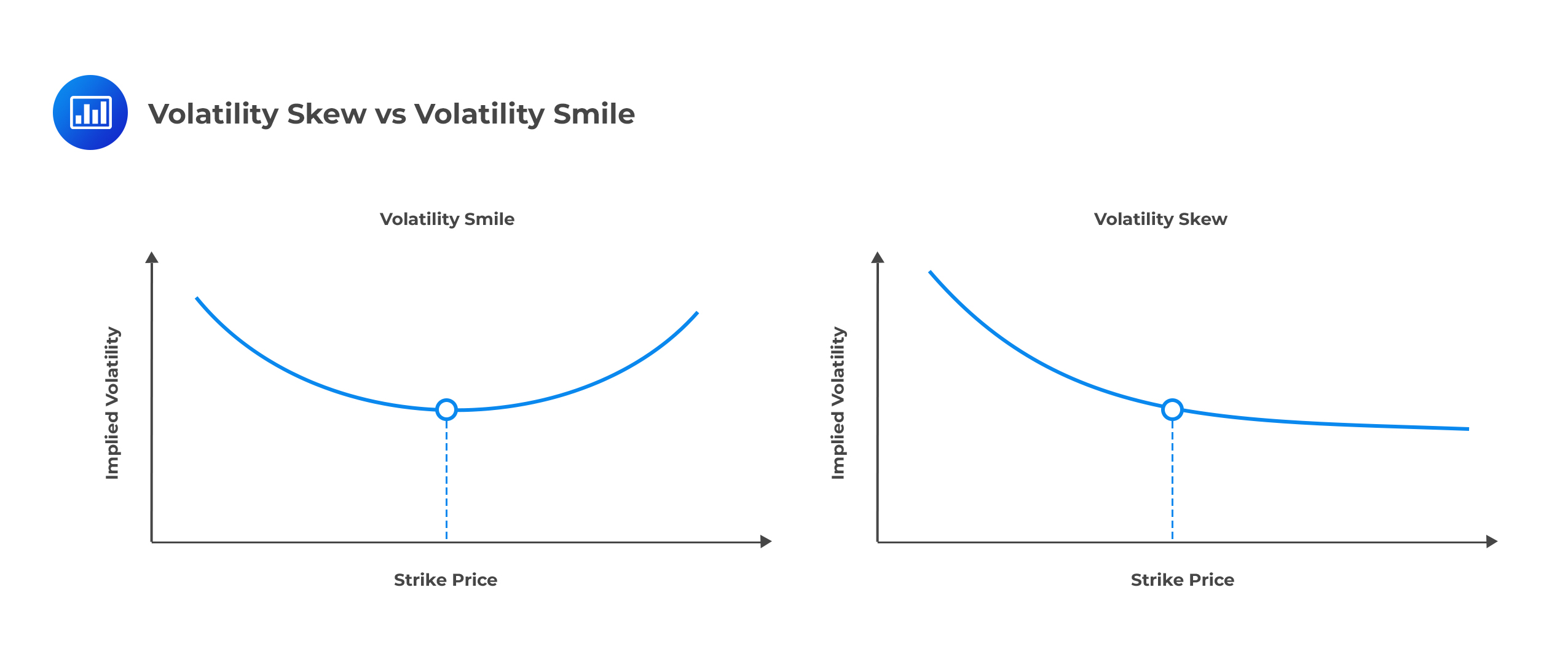
Volatility smiles are implied volatility patterns that arise in pricing financial options. When the implied volatility of options – with the same expiration date and the same underlying asset, but different strike prices – is graphed, the tendency is for that graph to show a smile. Going by the Black-Scholes option pricing model, we would expect a flat surface because volatility is assumed to be constant. (Note that Implied volatility captures a market’s forecast of a likely movement in a security’s price, unlike historical volatility which compares past market changes to their actual results. Options with high levels of implied volatility suggest that investors expect big moves in the underlying stocks. It could also signal that investors anticipate a major event that may trigger a big rally or a huge sell-off).

Volatility Skew

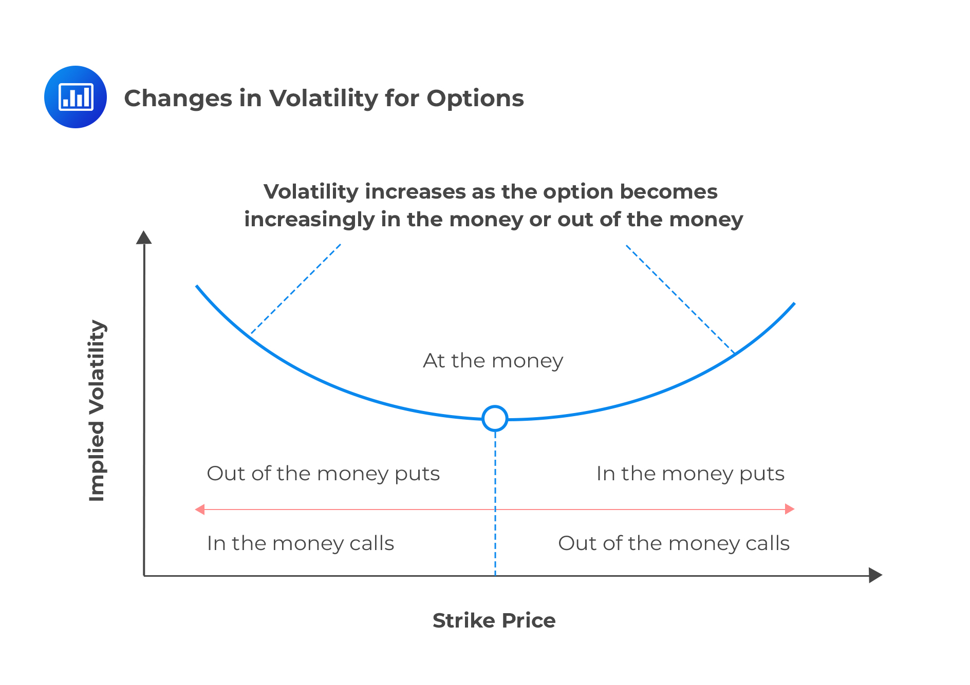
Volatility Skew is the difference in implied volatility among out-of-the-money options, at-the-money options, and in-the-money options. Implied volatility rises when the underlying asset of an option is further out-of-the-money (OTM) or in-the-money (ITM), compared to at-the-money (ATM). Options whose strike prices are at- or near-the-money have the lowest implied volatility.

The Implications of Put-Call Parity on the Implied Volatility of Call and Put Options

Put-call parity is a no-arbitrage equilibrium principle that relates European call and put options with the same underlying asset, strike price, and expiration date. It can be represented by the following relationship:

$$ \text{c} – \text p = \text S – \text{PV(X)} $$

where:

c = Price of a call.

p = Price of a put.

S = Price of the underlying security.

PV(X) = Present value of the strike.

Working with continuous time, the present value of the strike becomes:

$$ \text{PV(X)}=\text{Xe}^{-\text{rt}} $$

where r is the risk-free rate and t is the time left to expiration in years.

To determine the implications of put-call parity on the implied volatility of call and put options, we simply rearrange the put-call parity relationship and use subscripts alongside option prices to indicate whether they are market or Black-Scholes-Merton option prices. As a result, we generate the following pair of equations:

\(\text P_{\text {mkt}}+\text S_0 {\text e}^{-\text {qt}}=\text C_{\text {mkt}}+\text {PV}(\text X)\) ……………………equation I.

\(\text P_{\text {BSM}}+\text S_0 {\text e}^{-\text {qt}}=\text c_{\text {BSM}}+\text {PV(X)}\) …………………equation II.

Now, subtracting the second equation from the first one gives:

\(\text P_{\text {mkt}}-\text P_{\text {BSM}}=\text c_{\text {mkt}}-\text c_{\text {BSM}}\) ………………………equation III.

This relationship shows that, given the same strike price and time to expiration, the dollar pricing error when the Black-Scholes model is used to price a European put option should be exactly the same as the dollar pricing error when it is used to price a European call option. The implication is that the implied volatility of a call and put will be equal for the same strike price and time to expiration.

For purposes of illustration, let’s assume that we have a put option with an implied volatility of 25%. This means that \(\text P_{\text {mkt}}=\text P_{\text {BSM}}\) when a volatility of 25% is used in the Black–Scholes–Merton model. From equation III, it follows that \(\text c_{\text {mkt}}=\text c_{\text {BSM}}\) when this volatility is used. Therefore, the implied volatility of the call is also 25%. This shows that the implied volatility of a European call option is always the same as the implied volatility of a European put option when the two have the same strike price and maturity date.

Bottom line: The volatility smile (i.e., the relationship between implied volatility and strike price for a particular maturity) is the same for European calls and European puts.

As previously mentioned, the implied volatility is relatively low for at-the-money options. It becomes progressively higher as an option moves either into out of the money.

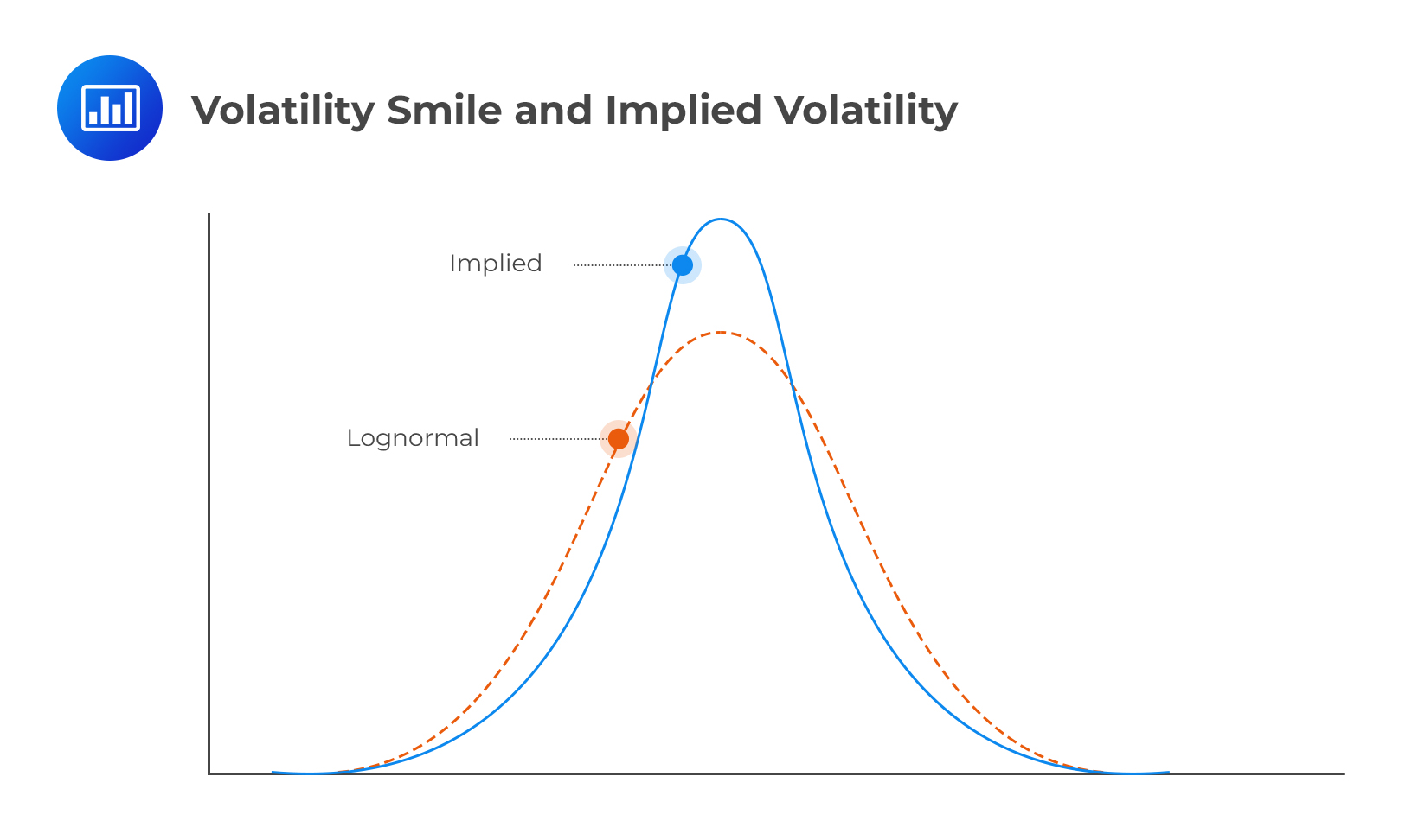
The volatility smile (i.e., the relationship between implied volatility and strike price for a particular maturity) corresponds to the implied distribution shown by the solid line in Figure 2. The dashed line shows a lognormal distribution with the same mean and standard deviation as the implied distribution. It is evident that the implied distribution has heavier tails than the lognormal distribution. Furthermore, the implied distribution is more peaked.

Characteristics of Foreign Exchange Rate Distributions and their Implications on Option Prices and Implied Volatility

Currency Options

The pattern for the implied volatility of currency options is such that it is higher for deep-in-the-money and deep-out-of-the-money options as compared to that of at-the-money options.

To see why this is the case, consider a call and a put on a certain currency pair, XY. The call has a positive payoff only if the actual exchange rate is above the strike rate. The put, on the other hand, has a positive payoff if the actual exchange rate is below the strike rate. If away-from-the-money exhibit greater implied volatility than at-the-money options, then it must be the case that currency traders anticipate a higher probability (greater chance) of extreme price movements than predicted by a lognormal distribution. This proposition is supported by empirical evidence.

Empirical Evidence

The following table demonstrates the daily movements in several different exchange rates over a period of time. The aim is to establish if traders are right to consider the lognormal distribution as understating the likelihood of extreme changes. We examine the daily movements in a total of 12 different exchange rates over a 10-year period. The steps taken to come up with the table are as follows:

• Step I:

  Calculating the standard deviation of daily percentage change in each exchange rate.

• Step II:

  Noting how often the actual percentage change exceeded 1 standard deviation, 2 standard deviations, and so on.

• Step III:

  Calculating how often this would have happened if the percentage changes had been normally distributed.

$$ \textbf{Percentage of days when Daily Exchange Rate Moves are Greater than} \\ \textbf{n Standard Deviations (n =1, 2, …. 5, 6)} $$

$$ \begin{array}{c|c|c} \textbf{Standard deviations} & \textbf{Real World} & \textbf{Lognormal Model} \\ \hline {>1 \text{ SD}} & {25.04} & {31.73} \\ \hline {>2 \text{ SD}} & {5.27} & {4.55} \\ \hline {>3 \text{ SD}} & {1.34} & {0.27} \\ \hline {>4 \text{ SD}} & {0.29} & {0.01} \\ \hline {>5 \text{ SD}} & {0.08} & {0.00} \\ \hline {>6 \text{ SD}} & {0.03} & {0.00} \\ \end{array} $$

In general, the percentage of days when daily exchange rate moves is greater than one, two, …, or six. Such standard deviations suggest a significant departure from the dictates of the lognormal distribution. For example, daily changes exceed 4, 5, and 6 standard deviations on 0.29%, 0.08%, and 0.03% of days, in that order. Note, however, that as per the lognormal model, we should hardly ever observe this happening. This proves the existence of heavy tails and presence of a volatility smile in currency options trading.

Extreme foreign exchange changes are possible only if the volatility is not constant. Note, however, that long-dated options tend to exhibit lower volatility compared to short-term options.

Equity Options

The equity option volatility pattern is different from the currency option smile. The pattern is more of a “smirk,” than a smile. This is an indication of a higher implied volatility for low strike price options (in-the-money calls and out-of-the-money puts) than for high strike price options (in-the-money puts and out-of-the-money calls).

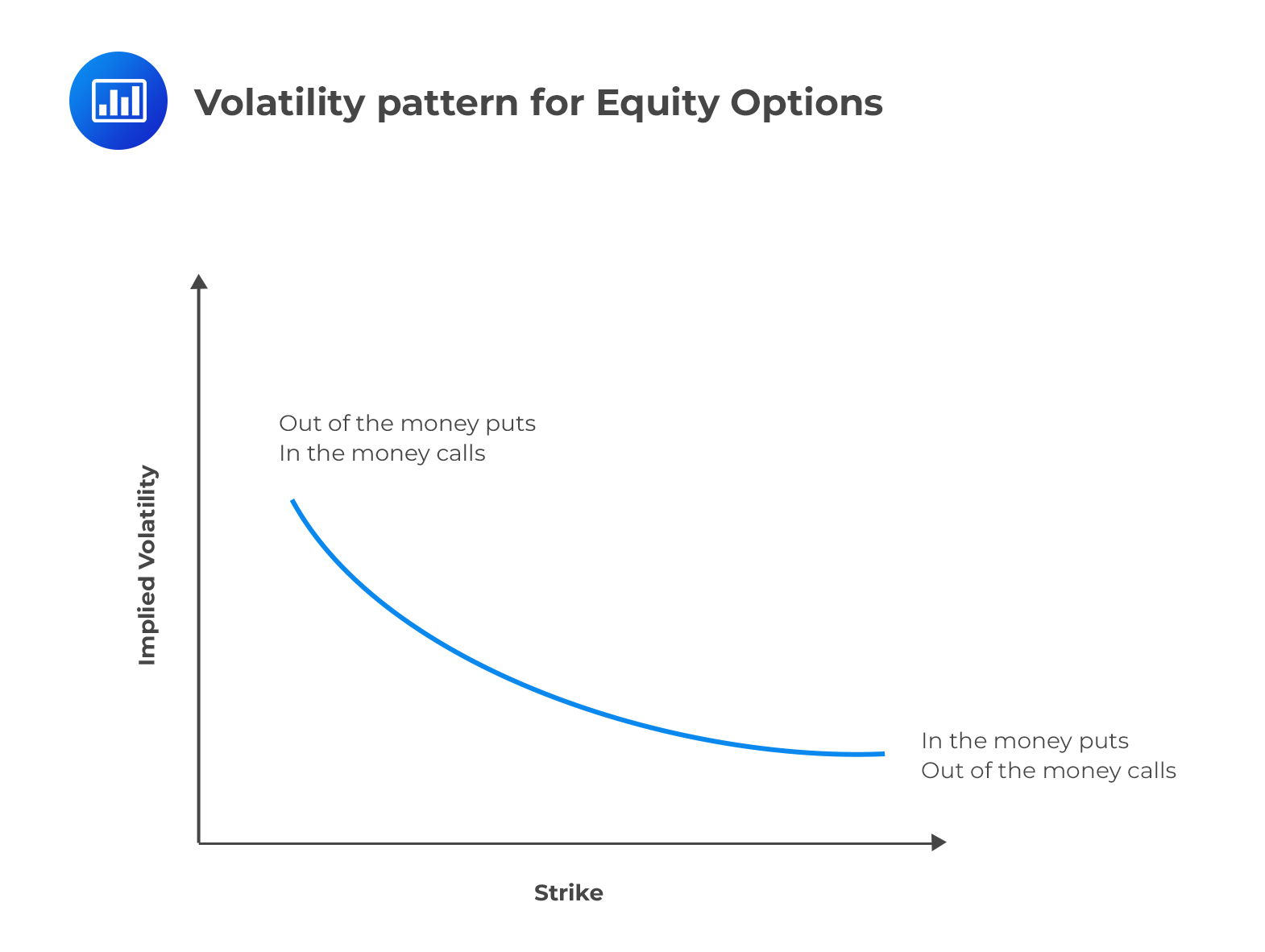The “smirk” (half-smile) suggests the existence of a left-skewed implied distribution of equity price changes. The implication is that traders believe that the probability of large down movements in price is greater than large up movements in price, as compared to a lognormal distribution.

There are two main reasons that explain the shape of the volatility smile for equity options:

1. Capital Structure Leverage

   An increase in a firm’s equity results in a decrease in leverage, which tends to decrease the riskiness of the firm. This lowers the volatility of the underlying asset. On the other hand, a decrease in a firm’s equity results in an increase in leverage, which makes the firm riskier. This increases the volatility of the underlying asset.

2. Crashophobia

   Literally, “crashophobia” refers to fears of a terrible crash. In 1987, there was a rapid downturn in stock markets that occurred over several days, causing massive losses to traders and investors around the globe. In the run-up to the crash, the Dow Jones Industrial Average (DJIA) registered hugely attractive returns. Since then, traders have been wary of a similar crash.

Crashophobia is synonymous with strong negative skewness in the physical stock returns distribution, suggesting that the probability of a large decrease in stock prices exceeds the probability of a large increase. As a result, traders feel more inclined to protect themselves from a downturn and therefore use put options as hedging instruments. The high demand for puts increases their prices (premium charged by option writers). In other words, deep out-of-the-money puts exhibit high premiums since they are seen as an insurance policy that protects against a substantial drop in equity prices. The ultimate result is a heavy left tail of the implied distribution.

Alternative Ways of Characterizing the Volatility Smile

So far, we have studied volatility patterns by examining the relationship between implied volatility and the strike price. In practice, traders also use alternative methods to study these volatility patterns. In almost all these alternatives, the strike price, which is essentially the independent variable, is replaced with other market parameters.

Alternative 1: Replacing the strike price X with strike price divided by stock price, \(\frac {\text X}{\text S_0}\).The resulting volatility smile is then more stable.

Alternative 2: Replacing the strike price with strike price divided by the forward price for the underlying asset, \(\frac {\text X}{\text F_0}\).This substitution is informed by the idea that traders usually define an option as at-the-money when K equals the forward price, \({\text F_0}\), not when it equals the spot price \({\text S_0}\)\).

Alternative 3: Replacing the strike price with the option’s delta. This approach allows the volatility smile to be applied to some non-standard options.

Volatility Term Structures and Volatility Surfaces

In addition to a volatility smile, traders use a volatility term structure when pricing options.

The volatility term structure is a listing of implied volatilities as a function of time to expiration for at-the-money option contracts. It is a curve depicting the differing implied volatilities of options with the same strike price but different maturities. By looking at term structures of implied volatility, investors are able to come up with a better expectation of whether an option expiring at time t will rise or fall in the future.

A rising term structure means that the implied volatility of long-term options is higher than that of short-term options. In these circumstances, traders would expect short-term implied volatility to rise. A falling term structure, on the other hand, means that the implied volatility of long-term options is lower than that of short-term options. In these circumstances, traders would expect the short-term volatility to fall.

Volatility surfaces combine volatility smiles with the volatility term structure to tabulate the volatilities appropriate for pricing an option with any strike price and any maturity.

As illustrated on figure 5, the shape of the volatility smile depends on the option maturity. Notably, the smile tends to become less pronounced (and more of a smirk) as the option maturity increases

$$ \textbf{Example of a Volatility Surface} $$

$$ \bf{\text{Volatility Smile} \left(\frac {\text K}{\text S_0} \right)} $$

$$ \begin{array}{c|c|c|c|c|c} {} & \bf{0.90} & \bf{0.95} & \bf{1.00} & \bf{1.05} & \bf{1.10} \\ \hline \textbf{Maturity} & {} & {} & {} & {} & {} \\ \hline \textbf{1 month} & {13.2} & {12.0} & {11.0} & {12.1} & {13.5} \\ \hline \textbf{3 months} & {13.0} & {12.0} & {11.0} & {12.1} & {13.1} \\ \hline \textbf{6 months} & {13.1} & {12.3} & {11.5} & {12.4} & {13.3} \\ \hline \textbf{1 year} & {13.7} & {13.0} & {12.5} & {13.0} & {13.8} \\ \hline \textbf{2 years} & {14.0} & {13.5} & {13.0} & {13.5} & {14.1} \\ \hline \textbf{5 years} & {13.8} & {13.7} & {13.5} & {13.6} & {14.0} \\ \end{array} $$

The Impact of the Volatility Smile on the Calculation of the “Greeks”

Option Greeks provide a way to measure the sensitivity of an option’s price to quantifiable factors.

Volatility smiles complicate the calculation of Greeks such as delta, vega, and gamma. In general, there are two rules that explain how implied volatility may affect the calculation of Greeks:

Rule #1 – Sticky Strike Rule

The sticky strike rule assumes that an option’s implied volatility is the same over short time periods (e.g., successive days). In other words, the implied volatility of an option remains constant from one day to the next. Going by this rule, the calculation of the Greeks is assumed to be unaffected as long as the implied volatility doesn’t change.

Rule #2 – Sticky Delta Rule

The sticky delta rule assumes that the relationship between an option price and the ratio of underlying to strike (S/K) is constant. In other words, it assumes that the volatility skew remains unchanged with moneyness.

For example, let’s assume that we are interested in an option on the S&P 500 index and that the implied volatility for an ATM option is 40% with the index level being at 3,000. Now, if the index declines to 2,900, the sticky delta rule would predict that the implied volatility for a 2,900 strike option would now be 40%. Therefore, this behavior is known as sticky moneyness or sticky delta.

The Impact of a Single Asset Price Jump on a Volatility Smile

Where a large jump—either up or down—is anticipated, the actual distribution is not lognormal but rather bimodal (two humps).

Example:

Let’s assume that a stock is currently priced at $300 and word on the street is that an important news announcement is due in a few days. Now, this announcement is expected either to increase the stock price by $20 or to reduce it by $20. In this scenario, the probability distribution of the stock price 1 month into the future might consist of a mixture of two lognormal distributions, one corresponding to favorable news, and the other corresponding to unfavorable news. This is illustrated below.

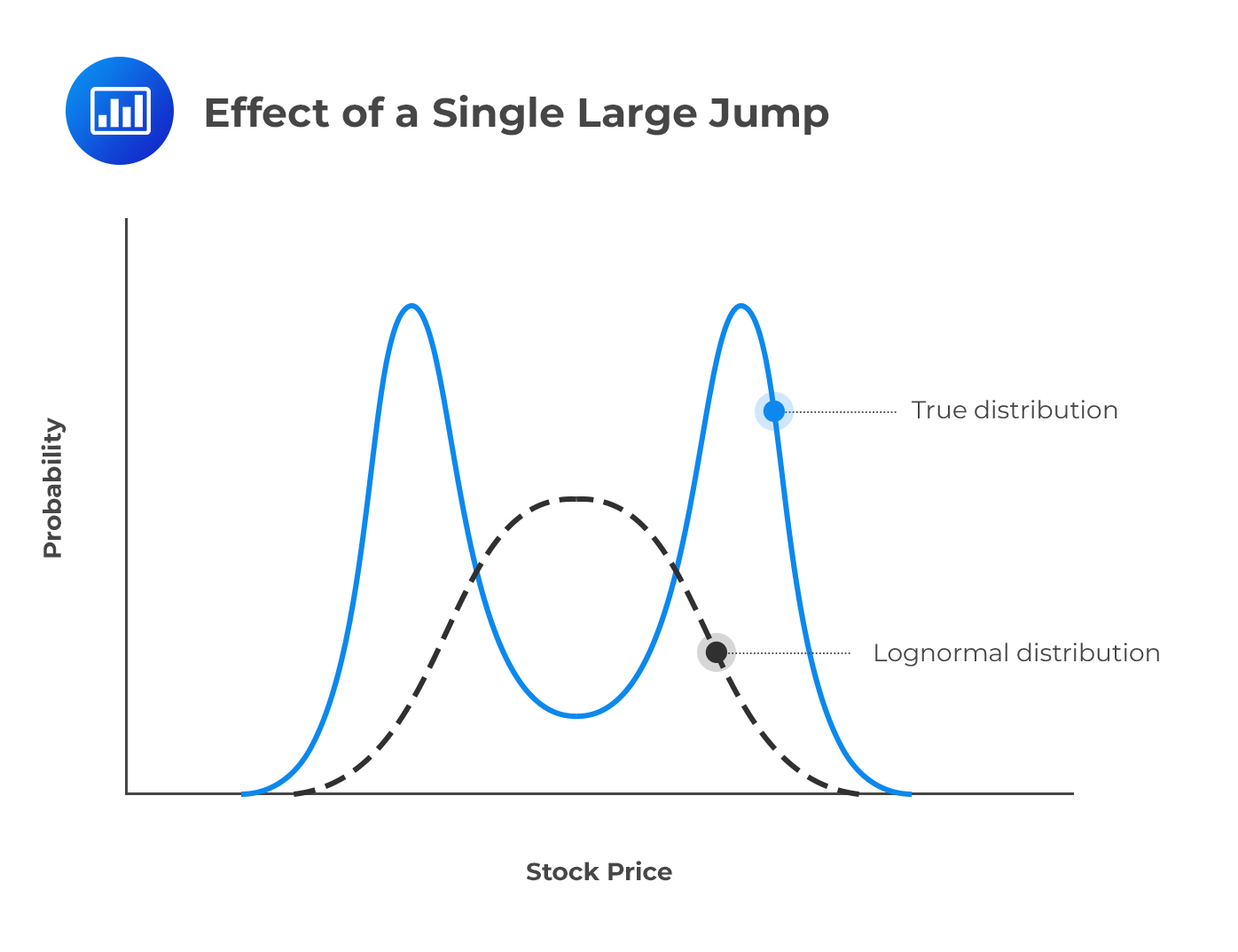Price jumps and the probabilities assumed for either a large up or down movement do affect the implied volatility of options. An at-the-money option has a higher volatility than both an out-of-the-money option and an in-the-money option. This generates an upside-down volatility smile that peaks in the middle.

Question 1

A foreign currency is valued at $200.71. The foreign currency has a European call option market price of $13.55 and a strike price of $225. In the US, the risk-free interest rate is 4% per annum and 7% per annum in the foreign country. Determine the price of a European put option with a 1-year maturity for the foreign currency.

1. $14.68.
2. $13.55.
3. $42.59.
4. $15.48.

The correct answer is C.

The price \(p\) of a European put option with a strike price of $1.60 and 1-year maturity must satisfy the following equation:

$$ p+{ S }_{ 0 }{ e }^{ -qT }=c+K{ e }^{ -rT } $$

From the question, we are provided that:

\({ S }_{ 0 }=$200.71\), \(q=16\%\), \(T=1\), \(c=13.55\), \(K=$225\) and \(r=7\%\)

Therefore:

$$\begin{align*} p+200.71\times { e }^{ -0.07\times 1 }&=13.55+225{ e }^{ -0.04\times 1 }\\ \Rightarrow p&=42.59\end{align*} $$

Question 2

\(g\left( { S }_{ T } \right) \) is a constant between \({ S }_{ T } =8\) and \({ S }_{ T }=10\). We are also informed that, a non-dividend paying stock has a price of $11.3 and a risk-free interest rate of 3%. The implied volatilities of 6-month European options with strike prices of $8, $9 and $10 are 13%, 12% and 10.5%, in that order. From Deriva Gem their prices are $2.35, $2.25 and $2.14, in that order, with \(K=7\) and \(\delta=0.32\). Compute the value of \({ g }_{ 1 }\) by interpolating to get the implied volatility of a 6-month option with a strike price of $8.50 as 12.6%.

1. 3.22.
2. 3.17.
3. 1.02.
4. 5.15.

The correct answer is B.

Note that:

$$ g\left( K \right) ={ e }^{ rt }\frac { { b }_{ 1 }+{ b }_{ 3 }-2{ b }_{ 2 } }{ { \delta }^{ 2 } } $$

From the problem, we have:

\(r=0.03\), \(t=0.5\), \({ b }_{ 1 }\), \({ b }_{ 2 }\) and \({ b }_{ 3 }\) are $2.35, $2.25 and $2.14, in that order.

Therefore:

$$\begin{align*} g\left( { S }_{ 1 } \right) &={ e }^{ 0.5\times 0.03 }\times \frac { \left( 2.35+2.25-2\times 2.14 \right) }{ { 0.32 }^{ 2 } }\\&=3.17 \end{align*}$$

Question 3

Assume that a foreign country \(X\) has its currency valued at $0.656. Suppose further that the European call and put options computed by Black-Scholes-Merton model are 0.0249 and 0.0501 respectively. Compute the market price of the call option if the market price of the put option is 0.0317.

1. 0.0056.
2. 0.0025.
3. 0.0337.
4. 0.0654.

The correct answer is A.

For Black-Scholes-Merton model and in the absence of arbitrage opportunities, the put-call parity satisfies:

$$ { p }_{ BS }+{ S }_{ 0 }{ e }^{ -qT }={ c }_{ BS }K{ e }^{ -rt } $$

For the market prices, put-call parity holds when arbitrage opportunities are absent such that:

$$ { p }_{ MKT }+{ S }_{ 0 }{ e }^{ -qT }={ c }_{ MKT }K{ e }^{ -rt } $$

The difference between the two equations is:

$$ { p }_{ BS }-{ p }_{ MKT }={ c }_{ BS }-{ c }_{ MKT } $$

From the question we have that:

\({ c }_{ BS }=0.0249\), \({ p }_{ BS }=0.051\) and \({ p }_{ MKT }=0.0317\)

Therefore:

$$\begin{align*} 0.051-0.0317&=0.0249-{ c }_{ MKT }\\ \Rightarrow { c }_{ MKT }&=0.0056 \end{align*}$$