Estimating Market Risk Measures

After completing this reading, you should be able to:

• Estimate VaR using a historical simulation approach.
• Estimate VaR using a parametric approach for both normal and lognormal return distributions.
• Estimate the expected shortfall given P/L or return data.
• Describe coherent risk measures.
• Estimate risk measures by estimating quantiles.
• Evaluate estimators of risk measures by estimating their standard errors.
• Interpre QQ plots to identify the characteristics of a distribution.

Estimating VaR Using a Historical Simulation Approach

One of the simplest approaches to estimating VaR involves historical simulation. In this case, a risk manager constructs a distribution of losses by subjecting the current portfolio to the actual changes in the key factors experienced over the last \(t\) time periods. After that, the mark-to-market P/L amounts for each period are calculated and recorded in an ordered fashion.

Let’s assume that we have a list of 100 ordered P/L observations and we would like to determine the VaR at 95% confidence. This implies that we should have a 5% tail, and that there are 5 observations (= 5% × 100) in the tail. In this scenario, the 95% VaR would be the \(\textbf {sixth largest}\) P/L observation.

In general, if there are \(\textbf {n ordered}\) observations, and a confidence level cl%, the cl% VaR is given by the \([(1 –cl\%) n + 1]^{th}\) highest observation. This is the observation that separates the tail from the body of the distribution. For instance, if we have 1,000 observations and a confidence level of 95%, the 95% VaR is given by the \((1 – 0.95)1,000 + 1 = 51^{st}\) observation. There are 50 observations in the tail.

Example: Computing VaR Using the Historical Simulation Approach

Over the past 300 trading days, the five worst daily losses (in millions) were: -30, -27, -23, -21, and -19. If the historical window is made up of these 300 daily P&L observations, what is the 99% daily HS VaR?

Solution

VaR is to be estimated at 99% confidence. This means that 1% (i.e., 3) of the ordered observations would fall in the tail of the distribution.

The 99% VaR would be given by the (1 – 0.99) 300 + 1 highest observation, i.e., the \(4^{\text{th}}\) highest value. This would be -21.

Note that the \(4^{\text{th}}\) highest observation would separate the 1% of the largest losses from the remaining 99% of returns.

Estimating Parametric VaR

When estimating VaR using the historical simulation approach, we do not make any assumption regarding the distribution of returns. In contrast, the parametric approach explicitly assumes a distribution for the underlying observations. We shall be looking at (1) VaR for returns that follow the normal distribution and (II) VaR for returns that follow the lognormal distribution.

1. Normal VaR

   1. Profit/Loss Data

      We have already established that the VaR for a given confidence level indicates the point that separates tail losses from the body of the distribution. Using P/L data, our VaR is:

      $$ \text{VaR}(\alpha\%)=-\mu_{\text{PL}}+\sigma_{\text{PL}}×z_{\alpha} $$

      where \(\mu_{\text{PL}}\)and \(\sigma_{\text{PL}}\) are the mean and standard deviation of P/L, and \(z_\alpha\) is the standard normal variate corresponding to the chosen confidence level. If we take the confidence level to be cl, then \(z_\alpha\) is the standard normal variate such that \(\text{cl}\) of the probability density function lies to the left, while \(1- \text{cl}\) of the probability density lies to the right. In most cases, you will be required to calculate the VaR when cl = 95%, in which case the standard normal variate is -1.645.

      Notably, the VaR cutoff will be on the left side of the distribution. As such, the VaR is usually negative but is reported as positive since it is the value that is at risk (the negative amount is implied).

      Example: Computing VaR (Normal Distribution)

      Let P/L for ABC limited over a specified period be normally distributed with a mean of $12 million and a standard deviation of $24 million. Calculate the 95% VaR and the corresponding 99% VaR.

      Solution

      $$ \begin{align*} 95\% \text{ VaR}: & \quad \alpha=95 \\ \text{VaR}(95\%) & =-\mu_{\text{PL}}+\sigma_{\text{PL}}×z_{95} \\ & =-12+24×1.645=27.48 \\ \end{align*} $$

      How do we interpret this? ABC \(\textbf{expects}\) to lose at most $27.48 million over the next year with 95% confidence. Equivalently, ABC \(\textbf{expects}\) to lose more than $27.48 million with a 5% probability.

      $$ \begin{align*} 99\% \text{ VaR}:&\quad \alpha=99 \\ \text{VaR}(99\%)&=-\mu_{\text{PL}}+\sigma_{\text{PL}}×z_{99} \\ & =-12+24×2.33=43.824 \\ \end{align*} $$ The 99% VaR can be interpreted in a similar fashion. However, note that the VaR at 99% confidence is significantly higher than the VaR at 95% confidence. Generally, the VaR increases as the confidence level increases.

   2. Arithmetic Data

      When using arithmetic data rather than P/L data, VaR calculation follows a similar format.

      Assuming the arithmetic returns follow a normal distribution,

      $$ {\text r}_{\text t}=\cfrac {\text p_{\text t}+{\text{D}_\text{t}}-\text p_{\text t-1}}{\text p_{\text t-1} } $$ Where \(\text p_\text t\): Asset price at the end of periods; \(\text D_{\text t}\): Interim payments

      The VaR is:

      $$ \text{VaR}(\alpha\%)=[-\mu_\text r+\sigma_\text r×z_\alpha ] \text p_{(\text t-1)} $$ \(\textbf{Example 1}: \textbf{Computing VaR given arithmetic data}\)

      The arithmetic returns \(r_t\), over some period of time, are normally distributed with a mean of 1.34 and a standard deviation 1.96. The portfolio is currently worth $1 million. Calculate the 95% VaR and 99% VaR.

      Solution

      $$ \begin{align*} \text {VaR}(\alpha \%) & =[-\mu_\text r+\sigma_\text r×z_\alpha ] \text p_{\text t-1} \\ 95\% \text{VaR}:& \quad \alpha=95 \\ \text{VaR}(95\%) & =[-1.34+1.96×1.645]×$1=$1.8842 \text{ million} \\ 99\% \text{ VaR}:& \quad \alpha=99 \\ \text {VaR}(99\%) & =[-1.34+1.96×2.33]×$1=$3.2190 \text{ million} \\ \end{align*} $$

      Again, note that as the confidence level increases, so does the VaR

      Example 2: Computing VaR Given Arithmetic Data

      A portfolio has a beginning period value of $200. The arithmetic returns follow a normal distribution with a mean of 15% and a standard deviation of 20%. Determine the VaR at both the 95% and 99% confidence levels.

      Solution

      $$ \begin{align*} \text{VaR}(\alpha\%) & =[-\mu_\text r+\sigma_\text r×\text z_\alpha ] \text p_{\text t-1} \\ 95\% \text{ VaR}:&\quad \alpha=95 \\ \text{VaR}(95\%)& =[-0.15+0.2×1.645]×$200=$35.8 \text{ million} \\ 99\% \text { VaR}:&\quad \alpha=99 \\ \text{VaR}(99\%)&=[-0.15+0.2×2.33]×$200=$63.2 \text{ million} \\ \end{align*} $$

2. Lognormal VaR

   Unlike the normal distribution, the lognormal distribution is bounded by zero. Besides, it is also skewed to the right.

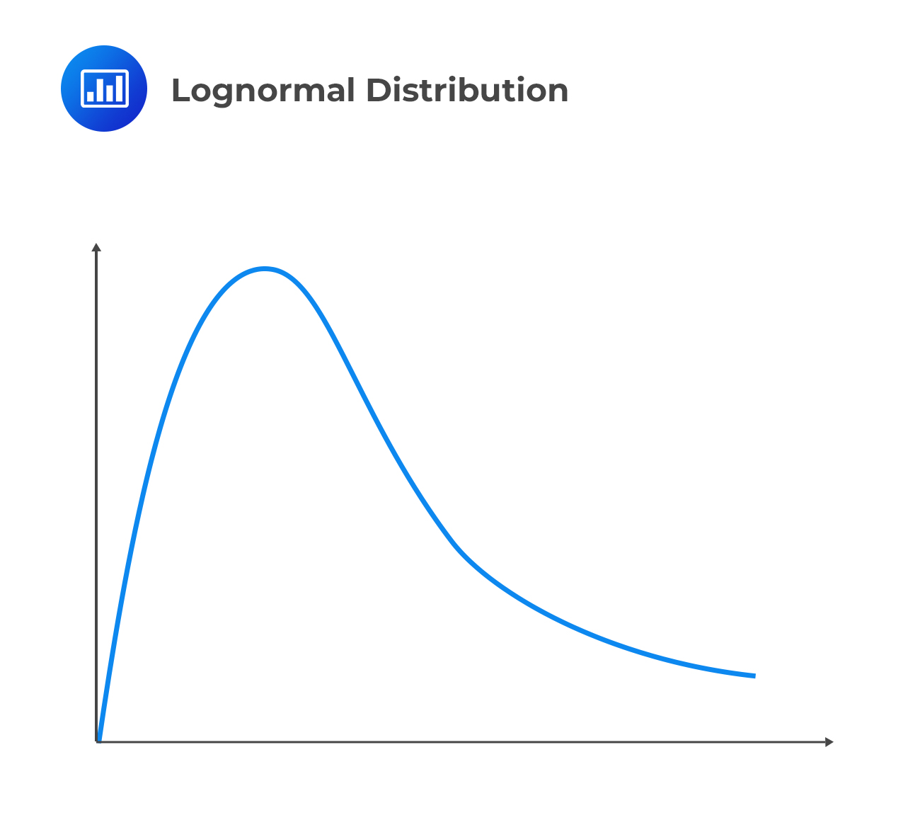   This explains why this is the favored distribution when modeling the prices of assets such as stocks (which can never be negative). We also ditch the arithmetic returns in favor of geometric ones. As earlier established, the geometric return is:

   $$ \text R_\text t=\text{ln}⁡ \left[ \cfrac {\text p_\text t+\text D_\text t}{\text p_{\text t-1}} \right] $$

   If we assume that geometric returns follow a normal distribution \((\mu_\text R, \sigma_\text R)\), then the natural logarithm of asset prices follows a normal distribution and \(\text p_\text t\) follows a lognormal distribution

   It can be shown that:

   $$ \text{VaR}(\alpha \%)=(1-\text e^{\mu_\text R-\sigma_\text R×\text z_\alpha } ) \text p_{\text t-1} $$

   Example: Computing Lognormal VaR

   Assume that geometric returns over a given period are distributed as normal with a mean of 0.1 and standard deviation of 0.15, and we have a portfolio currently valued at $20 million. Calculate the VaR at both 95% and 99% confidence.

   Solution

   $$ \begin{align*} \text{VaR}(\alpha \%) & =(1-\text e^{\mu_\text R-\sigma_\text R×\text z_\alpha } ) \text p_{(\text t-1)} \\ 95\% \text{ VaR}:& \quad \alpha=95 \\ \text{VaR}(95\%) &=(1-e^{0.1-0.15×1.645} )20=$2.7298 \text{ million} \\ 99\% \text{ VaR}:& \quad \alpha=99 \\ \text{VaR}(99\%) &=(1-e^{0.1-0.15×2.33} )20=$4.4162 \text{ million} \\ \end{align*} $$

   Example 2: Computing Lognormal VaR

   Let’s assume that the geometric returns Rt, are distributed as normal with a mean 0.06 and standard a deviation 0.30. The portfolio is currently worth $1 million. Calculate the 95% and 99% lognormal VaR.

   Solution

   $$ \begin{align*} \text{VaR}(\alpha\%)&=(1-\text e^{\mu_\text R-\sigma_\text R×\text z_\alpha } ) \text p_{(\text t-1)} \\ 95\% \text{ VaR}:& \quad \alpha=95 \\ \text{VaR}(95\%)&=(1-\text e^{0.06-0.30×1.645} )1=$0.3518 \text{ million} \\ 99\% \text{ VaR}:& \quad \alpha=99 \\ \text{VaR}(99\%)& =(1-e^{0.06-0.30×2.33} )1=$0.4689 \text{ million} \end{align*} $$

Estimating the Expected Shortfall Given P/L or Return Data

Despite the significant role VaR plays in risk management, it stops short of telling us the amount or magnitude of the actual loss. What it tells us is the maximum value we stand to lose for a given confidence level. If the 95% VaR is, say, $2 million, we would expect to lose not more than $2 million with 95% confidence. However, we do not know what amount the actual loss would be. To have an idea of the magnitude of the expected loss, we need to compute the expected shortfall.

Expected shortfall (ES) is the expected loss given that the portfolio return already lies below the pre-specified worst-case quantile return, e.g., below the 5th percentile return. Put differently, expected shortfall is the mean percent loss among the returns found below the q-quantile (q is usually 5%). It helps answer the question: If we experience a catastrophic event, what is the expected loss in our financial position?

The expected shortfall (ES) provides an estimate of the tail loss by averaging the VaRs for increasing confidence levels in the tail. It is also called the \(\textbf{expected tail loss }\)(ETL) or the \(\textbf{conditional VaR}\).

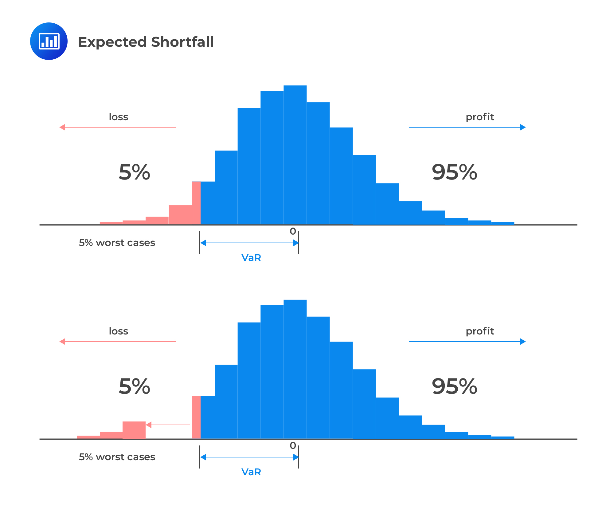To determine the ES, the tail mass is divided into \(\textbf{n equal slices}\) and the corresponding n – 1 VaRs are computed.

Illustration

Assume that we wish to estimate a 95% ES on the assumption that losses are normally distributed with a mean of 0 and a standard deviation of 1. Ideally, we would need a large value of n to improve accuracy and reliability and then use the appropriate computer software. For illustration purposes, however, let’s assume that n = 10.

This value gives us 9 tail VaRs (i.e., 10 – 1) at confidence levels in excess of 95%. These vaRs are listed below. The estimated ES is the \(\textbf{average}\) of these VaRs.

$$ \begin{array}{c|c} \textbf{Confidence level} & \textbf{Tail VaR} \\ \hline {95.5\%} & {1.6954} \\ \hline {96.0\%} & {1.7507} \\ \hline {96.5\%} & {1.8119} \\ \hline {97.0\%} & {1.8808} \\ \hline {97.5\%} & {1.9600} \\ \hline {98.0\%} & {2.0537} \\ \hline {98.5\%} & {2.1701} \\ \hline {99.0\%} & {2.3263} \\ \hline {99.5\%} & {2.5738} \\ \hline {} & {\text{Average of tail VaRs} = \text{ES} =} \\ {} & {2.0250} \\ \end{array} $$

The theoretical true value of the ES can be worked out by using different values of n. This can easily be achieved with the help of computer software.

$$ \begin{array}{c|c} {\textbf{Number of tail slices }(\textbf n)} & \textbf{ES} \\ \hline {10} & {2.0250} \\ \hline {25} & {2.0433} \\ \hline {50} & {2.0513} \\ \hline {100} & {2.0562} \\ \hline {250} & {2.0597} \\ \hline {500} & {2.0610} \\ \hline {1,000} & {2.0618} \\ \hline {2,500} & {2.0623} \\ \hline {5,000} & {2.0625} \\ \hline {10,000} & {2.0626} \\ \hline {} & {\text{Theoretical average} =} \\ {} & {2.063} \\ \end{array} $$

These results show that the estimated ES rises with n and gradually converges at the theoretical true value of 2.063.

Example: Computing the Expected Shortfall Given P/L Data

A market risk manager uses historical information on 300 days of profit/loss information and calculates a VaR, at the 95th percentile, of CAD30 million. Loss observations beyond the 95th percentile are then used to estimate the expected shortfall. These losses(in millions) are CAD23, 24, 26, 28, 30, 33, 37, 42, 46, and 47. What is the conditional VaR?

Solution

Expected shortfall is the average of tail losses.

$$ \begin{align*} \text{ES} & =\left( \cfrac {23+24+26+28+30+33+37+42+46+47}{10} \right) \\ & =\text{CAD }33.6 \text{ million} \\ \end{align*} $$

Coherent Risk Measures

If X and Y are the future values of two risky positions, a risk measure \(\rho(\bullet )\) is said to be coherent if it satisfies the following properties:

1. Sub-additivity: \(\rho(X + Y ) \le \rho(X) + \rho(Y )\)

   Interpretation: If we add two portfolios to the total risk, the risk measure can’t get any worse than adding the two risks separately.

2. Homogeneity: \(\rho(XX) = X\rho(X)\)

   Interpretation: Doubling a portfolio consequently doubles the risk.

3. Monotonicity: \(\rho(X) \ge \rho(Y ), \text{ if } X \le Y\)

   Interpretation: If one portfolio has better values than another under all scenarios then its risk will be better.

4. Translation invariance: \(\rho(X + n) = \rho(X) –n\)

   Interpretation: the addition of a sure amount n (cash) to our position will decrease our risk by the same amount because it will increase the value of our end-of-period portfolio.

VaR is not a coherent risk measure because it fails to satisfy the sub-additivity property. The expected shortfall (ES), however, does satisfy this property and is, therefore, a coherent risk measure. If we combine two portfolios, the total ES would usually decrease to reflect the benefits of diversification. The ES would certainly \(\textbf{never}\) increase because it takes correlations into account. By contrast, the total VAR \(\textbf{can}\) – and in fact occasionally does – increase. As a result, the ES does not discourage risk diversification, but the VaR sometimes does.

The ES tells us what to expect in bad (i.e., tail) states—it gives an idea of how bad it might be, whilst the VaR tells us nothing other than to expect a loss higher than the VaR itself.

The ES is also better justified than VAR in terms of decision theory.

Assume that you are faced with a choice between two portfolios, A and B, with different distributions. Under \(\textbf{first}-\textbf{order stochastic dominance }\)(FSD) which is a rather strict decision rule, A has first-order stochastic dominance over random variable B if, for any outcome x, A gives at least as high a probability of receiving at least x as does B, and for some x, A gives a higher probability of receiving at least x. And under \(\textbf{second}-\textbf{order stochastic dominance}\) (SSD), a more realistic decision rule, portfolio A would dominate B if it has a higher mean and lower risk. Using the

ES as a risk measure is consistent with SSD, whereas VAR requires FSD, which is less realistic.

Overall, the ES dominates the VaR and presents a stronger case for use in risk management.

Estimating Risk Measures by Estimating Quantiles

It is possible to estimate coherent risk measures by manipulating the “average VaR” method. A coherent risk measure is a weighted average of the quantiles (denoted by \({ q }_{ p }\) of the loss distribution):

$$ { M }_{ \emptyset }=\int _{ 0 }^{ 1 }{ \emptyset \left( p \right) { q }_{ p } } dp $$

where the weighting function \({ \emptyset }(p)\) is specified by the user, depending on their risk aversion. The ES gives all tail-loss quantiles an equal weight of [1/(1 – cl)] and other quantiles a weight of 0. Therefore, the ES is a special case of \(M_{ \emptyset }\).

Under the more general coherent risk measure, the entire distribution is divided into equal \(\textbf{probability slices weighted by the more general risk aversion}\) (weighting) function.

We could illustrate this procedure for n = 10. The first step is to divide the entire return distribution into nine (10 – 1) equal probability mass slices (loss quantiles) as shown below. Each breakpoint indicates a different quantile.

For example, the 10% quantile(confidence level = 10%) relates to -1.2816, the 30% quantile (confidence level = 30%) relates to -0.5244, the 50% quantile (confidence level = 50%) relates to 0.0,and the 90% quantile (confidence level = 90%) relates to 1.2816. After that, each quantile is \(\textbf{weighted}\) by the specific risk aversion function and then \(\textbf{averaged}\) to arrive at the value of the coherent risk measure.

$$ \begin{array}{c|c|c|c} {\textbf{Confidence Level}} & {\textbf{Normal Deviate }(\textbf A)} & {\textbf{Weight }(\textbf B)} & {\textbf A × \textbf B} \\ \hline {10\%} & {-1.2816} & {0} & {} \\ \hline {20\%} & {-0.8416} & {0} & {} \\ \hline {30\%} & {-0.5244} & {0} & {} \\ \hline {40\%} & {-0.2533} & {x} & {} \\ \hline {50\%} & {0.0} & {xx} & {} \\ \hline {60\%} & {0.2533} & {xxx} & {} \\ \hline {70\%} & {0.5244} & {xxxx} & {} \\ \hline {80\%} & {0.8416} & {xxxxx} & {} \\ \hline {90\%} & {1.2816} & {xxxxxx} & {} \\ \hline {} & {} & {} & {\text{Average risk measure}} \\ {} & {} & {} & {= \text{sum of A} × \text B} \\ \end{array} $$

The xs in the third column represent weight that depends on the investor’s risk aversion.

Compared to the expected shortfall, such a coherent risk measure is more sensitive to the choice of n. However, as n increases, the risk measure converges at its true value. Remember that increasing the value of n takes us farther into some very extreme values at the tail.

Evaluating Estimators of Risk Measures by Estimating Their Standard Errors

Bear in mind that any risk measure estimates are only as useful as their precision. The true value of any risk measure is unknown and therefore, it is important to come up with estimates in a precise manner. Why? Only then can we be confident that the true value is fairly close to the estimate. Hence, it is important to supplement risk measure estimates with some indicator that gauges their precision. The standard error is a useful indicator of precision. More generally, confidence intervals (built with the help of standard errors) can be used.

The big question is: How do we go about determining standard errors and establishing confidence intervals? Let’s start with a sample size of n and arbitrary bin width of h around quantile, q. Bin width refers to the width of the intervals, or what we usually call “bins,” in a (statistical) histogram. The square root of the variance of the quantile is equal to the standard error of the quantile. Once the standard error has been specified, a confidence interval for a risk measure can be constructed:

$$ [ q+se(q)×z_\alpha ] > \text{VaR}>[q-se(q)×z_\alpha ] $$

Example: Computing the Standard Error for a Risk Measure

Construct a 90% confidence interval for 5% VaR (the 95% quantile) drawn from a standard normal distribution. Assume bin width = 0.1 and that the sample size is equal to 1,000.

Solution

Step 1: Determine the value of q.

The quantile value, q, corresponds to the 5% VaR. For the normal distribution, the 5% VaR occurs at 1.645 (implying that q = 1.645). So in crude form, the confidence interval will take the following shape:

$$ [q+se(q)×z_\alpha ]> \text{VaR} > [q-se(q)×z_\alpha ] $$

Step 2: Determine the range of q.

For the bin width of 0.1, we know that q falls in the bin spanning 1.645 \(\pm\) 0.1/2 = [1.595,1.695].

Note: The left tail probability, p, is the area to the left of 1.695 for a standard normal distribution.

Step 3: Determine the probability mass f(q).

We wish to calculate the probability mass between 1.595 and 1.695, represented as f(q). From the normal distribution table, the probability of a loss exceeding 1.695 is 4.5% (which is also equal to p) and the probability of profit or a loss less than 1.595 is 94.46%. Hence, f(q) = 1 – 0.045 – 0.9446 = 1.032%.

Step 4: Calculate the standard error of the quantile from the variance approximation of q.

$$ se(q)=\cfrac {\sqrt{\cfrac {p(1-p)}{n}}}{f(q)} $$ In this case, $$ se(q)=\cfrac {\sqrt{\cfrac {0.045×0.955}{1000}}}{0.01032}=0.63523 $$ Therefore, the following gives us the required CI: $$ \begin{align*} & [1.645+0.63523×1.645] > \text{VaR} > [1.645-0.63523×1.645] \\ & =2.69 > VaR > 0.6 \\ \end{align*} $$

Important:

Unlike the VaR, confidence intervals are two-sided. So, for a 90% CI, there will be 5% in each tail. This is equivalent to the 5% significance level of VaR, and as such, the critical values are \(\pm\)1.645.

The larger the sample size, the smaller the standard error, and the narrower the confidence interval.

Increasing the bin size, h, holding all else constant, will increase the probability mass f(q) and reduce p, the probability in the left tail. Subsequently, the standard error will decrease and the confidence interval will again narrow.

Increasing p implies that tail probabilities are more likely. When that happens, the estimator becomes less precise, and standard errors increase, widening the confidence interval. Note that the expression p(1- p) will be maximized at p = 0.5.

Interpreting QQ Plots to Identify the Characteristics of a Distribution

The quantile-quantile plot, more commonly called the Q-Q plot, is a graphical tool we can use to assess if a set of data plausibly came from some theoretical distributions such as a Normal or exponential.

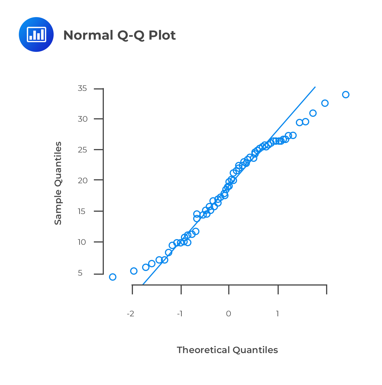For example, if we conduct risk analysis assuming that the underlying data is normally distributed, we can use a normal QQ plot to check whether that assumption is valid. We would need to plot the quantiles of our data set against the quantiles of the normal distribution. It’s not a perfect air-tight verification modality but a visual proof that can be quite subjective.

Remember that by a quantile, we mean the fraction (or percentage) of points below a given value. For example, the 0.1 (or 10%) quantile is the point at which 10% percent of the data fall below and 90% fall above that value.

Why are QQ Plots Important?

To start with, we can use a QQ plot to form a tentative view of the distribution from which our data might be drawn. This involves specification of a variety of alternative distributions and construction of QQ plots for each. If the data are drawn from the reference population, then the QQ plot should be linear. Any reference distributions that produce non-linear QQ plots can then be dismissed, and any distribution that produces a linear QQ plot is a good candidate distribution for our data.

In addition, since a linear transformation in one of the distributions in a QQ plot changes the intercept and slope of the QQ plot we can use the intercept and slope of a linear QQ plot to give us a rough idea of the location and scale parameters of our sample data.

Ultimately, if the empirical distribution has heavier tails than the reference distribution, the QQ plot will have steeper slopes at its tails, even if the central mass of the empirical observations is approximately linear.

In conclusion, a QQ plot is good for identifying outliers (e.g., observations contaminated by large errors).

Illustration

The chart here shows a QQ plot for a data sample drawn from a normal distribution, compared to a reference distribution that is also normal. The central mass observations fit a linear QQ plot very closely while the observations at the tail are a bit spread out. In this case, the empirical distribution matches the reference population.

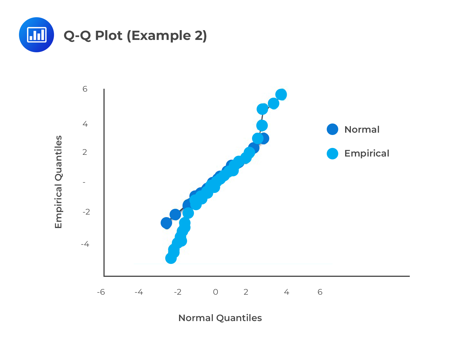
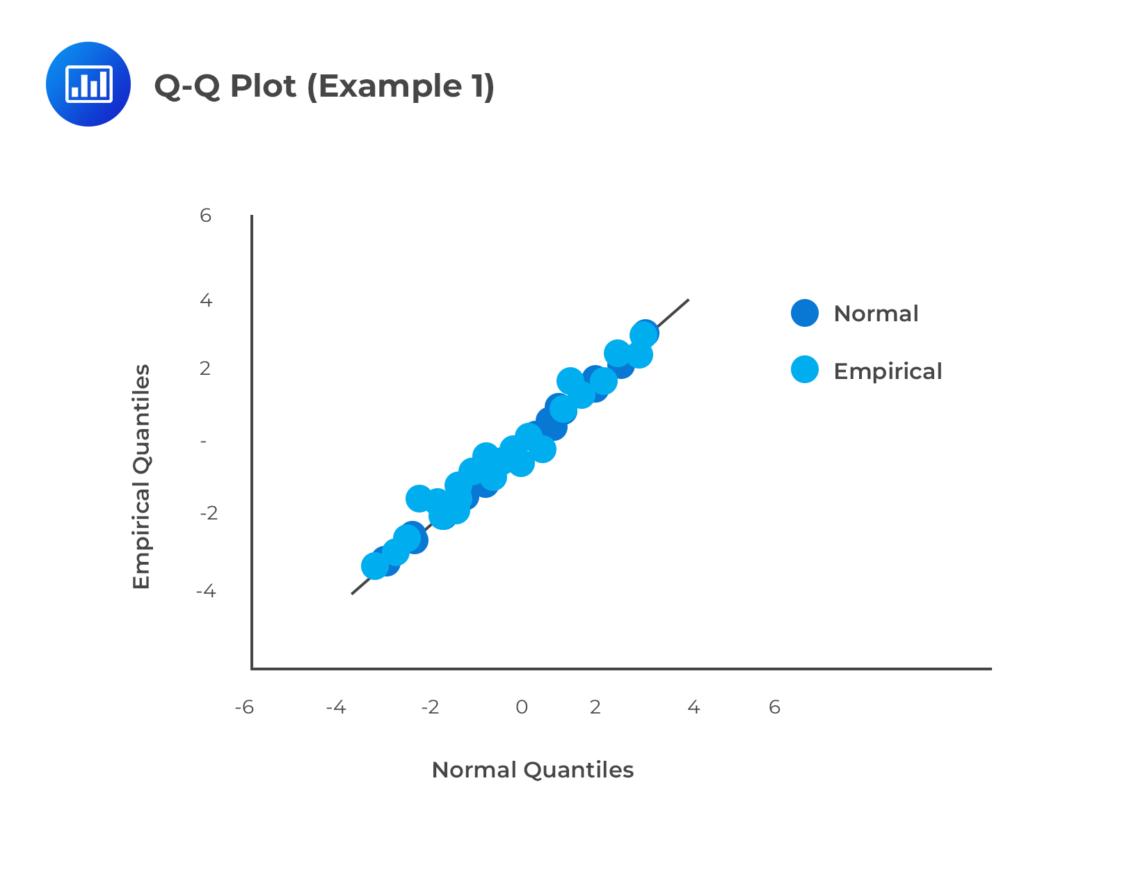The next one shows a QQ plot for a data sample drawn from a normal distribution, compared to a reference distribution that is \(\textbf{not}\) normal. Notably, it has a very heavy left tail and light right tail. In this case, the empirical distribution does not match the reference population.

Practice Questions

Question 1

If the arithmetic returns \({ r }_{ t }\) over some period of time are 0.075, what are the geometric returns?

1. -2.59.
2. 0.0723.
3. 0.0779.
4. 0.0895.

The correct answer is B.

Recall that,\( { R }_{ t }=ln\left( 1+{ r }_{ t } \right) \)

Therefore, \(ln(1+.075) = ln(1.075) = 0.0723\)

Question 2

Let the geometric returns \({ r }_{ t }\) be 0.020, over a specified period, calculate the arithmetic returns.

1. 0.1823.
2. 0.0182.
3. 0.0202.
4. 0.2020.

The correct answer is C.

Recall, \(1+{ r }_{ t }=exp({ R }_{ t })\), then: \({ r }_{ t }=exp({ R }_{ t })-1\)

Implying that: \(exp(0.020) – 1 = 0.0202\)

Question 3

Assuming that \(P/L\) over a specified period is normally distributed and has a mean of 13.9 and a standard deviation of 23.1. What is the 95% \(VaR\)?

1. 24.22.
2. 25.10.
3. 51.90.
4. 59.18.

The correct answer is A.

Recall that: \(\alpha VaR=-{ \mu }_{ P/L }+{ \sigma }_{ P/L }{ z }_{ \alpha , }\)

95% \(VaR\) is: \(-13.9+23.1{ Z }_{ 0.95 }=-13.9+23.1\times 1.65=24.22\)

Question 4

The arithmetic returns \({ r }_{ t }\), over some period of time, are normally distributed with a mean of 1.89 and a standard deviation 0.98. The portfolio is currently worth $1. Calculate the 99% \(VaR\).

1. 0.3895.
2. 4.1695.
3. 3.8108.
4. 0.0308.

The correct answer is A.

Remember that, \(\alpha VaR=-({ \mu }_{ r }-{ \sigma }_{ r }{ z }_{ \alpha }){ P }_{ t-1 }\),

99% \(VaR\) : \(-1.89+0.98\times 2.326=0.3895\)

Question 5

Assuming we make the empirical assumption that the mean and volatility of annualized returns are 0.24 and 0.67. Further, assuming there are 250 trading days in the years, calculate the normal 95% \(VaR\) and lognormal 95% \(VaR\) at the 1-day holding period for a portfolio worth $1.

A. 95% \(VaR\): 6.89%; lognormal 95% \(VaR\): 6.11%.

B. 95% \(VaR\): 6.89%; lognormal 95% \(VaR\): 6.65%.

C. 95% \(VaR\): 6.65%; lognormal 95% \(VaR\): 6.11%.

D. 95% \(VaR\): 6.65%; lognormal 95% \(VaR\): 6.04%.

The correct answer is B.

The daily return has a mean \(0.24/250 = 0.00096\) and standard deviation \(0.67/\sqrt { 250 } =0.0424 \).

Then, the normal 95% \(VaR\) is \(-0.00096+0.0424\times 1.645=0.0689\).

Therefore, the normal \(VaR\) is 6.89%.

If we assume a lognormal, then the 95% \(VaR\) is \(1-exp(0.00096-0.0424\times 1.645)=0.0665\).

This implies that the lognormal \(VaR\) is 6.65% of the value of the portfolio.