Stationary Time Series

After completing this reading, you should be able to:

• Describe the requirements for a series to be covariance stationary.
• Define the autocovariance function and the autocorrelation function.
• Define white noise; describe independent white noise and normal (Gaussian) white noise.
• Define and describe the properties of autoregressive (AR) processes.
• Define and describe the properties of moving average (MA) processes.
• Explain how a lag operator works.
• Explain mean reversion and calculate a mean-reverting level.
• Define and describe the properties of autoregressive moving average (ARMA) processes.
• Describe the application of AR, MA, and ARMA processes.
• Describe sample autocorrelation and partial autocorrelation.
• Describe the Box-Pierce Q-statistic and the Ljung-Box Q statistic.
• Explain how forecasts are generated from ARMA models.
• Describe the role of mean reversion in long-horizon forecasts.
• Explain how seasonality is modeled in a covariance-stationary ARMA.

Time series is a collection of observations on a variable’s outcome in distinct periods — for example, monthly sales of a company for the past ten years. Time series are used to forecast the future of the time series. The time series are classified into the trend, seasonal, and cyclical components. A trend time-series changes its level over time, while a seasonal time series has predictable changes over a given time. Lastly, a cyclical time series, as its name suggests, reflects the cycles in a given data. We will concentrate on the cyclical data (especially linear stochastic processes).

A stochastic process is a set of variables. The stochastic process is mostly denoted by \(Y_t\) and by the subscript, the random variable is ordered time so that \(Y_s\) occurs first before \(Y_t\) if \(s<t\).

A linear process has a general form of:

$$ \begin{align*} Y_t & =α_t+β_0 ϵ_t+β_1 ϵ_{t-1}+β_2 ϵ_{t-2}+…\\ & ={\alpha}_t +\sum_{i=0}^{\infty}{{\beta}_i}{\epsilon}_{t-i} \\ \end{align*} $$

The linear process is linear on the shock, \(ϵ_t\). \(α_t\) is a deterministic while \(β_i\) is a constant coefficient.

Covariance Stationary Time Series

The ordered set: \(\left\{ \dots ,{ y }_{ -2 },{ y }_{ -1 },{ y }_{ 0 },{ y }_{ 1 },{ y }_{ 2 },\dots \right\} \) is called the realization of a time series. Theoretically, it starts from the infinite past and proceeds to the infinite future. However, only a finite subset of realization can be used in practice, and is called a sample path.

A series is said to be covariance stationary if both its mean and covariance structure is stable over time.

More specifically, a time series is said to be covariance stationary if:

I. The mean does not change and thus constant over time. That is:

$$E(Y_t )=μ ∀t$$

II. The variance does change over time, and it is constant. That is:

$$V(Y_t )=γ_0 <∞ \ ∀t$$

III. The autocovariance of the time series is finite and does not change over time, and it depends on the distance between two observations. That is:

$$Cov\left(Y_t,Y_{t-h}\right)=γ_h ∀t$$

The covariance stationarity is crucial so that the time series has a constant relationship across time and that the parameters are easily interpreted since the parameters will be asymptotically normally distributed.

Autocovariance and Autocorrelation Functions

The Autocovariance Function

It can be quite challenging to quantify the stability of a covariance structure. We will, therefore, use the autocovariance function. The autocovariance is the covariance between the stochastic process at a different point in time (analogous to the covariance between two random variables). It is given by:

$$γ_{t,h}=E\left[\left(Y_t – E\left(Y_t \right)\right)\left(Y_{t-h}-E\left(Y_{t-h} \right)\right)\right]$$

And if the length \(h=0\) then:

$$γ_{t,h}=E\left[\left(Y_t-E(Y_t )\right)^2\right]$$

Which is the variance of \(Y_t\).

The autocovariance is a function of \(h\) so that:

$$γ_h=γ_{|h|}$$

This is asserting the fact that the autocovariance depends on the length \(h\) and not the time \(t\). So that:

$$Cov \left(Y_t,Y_{t-h}\right)=Cov\left(Y_{t-h}, Y_t\right)$$

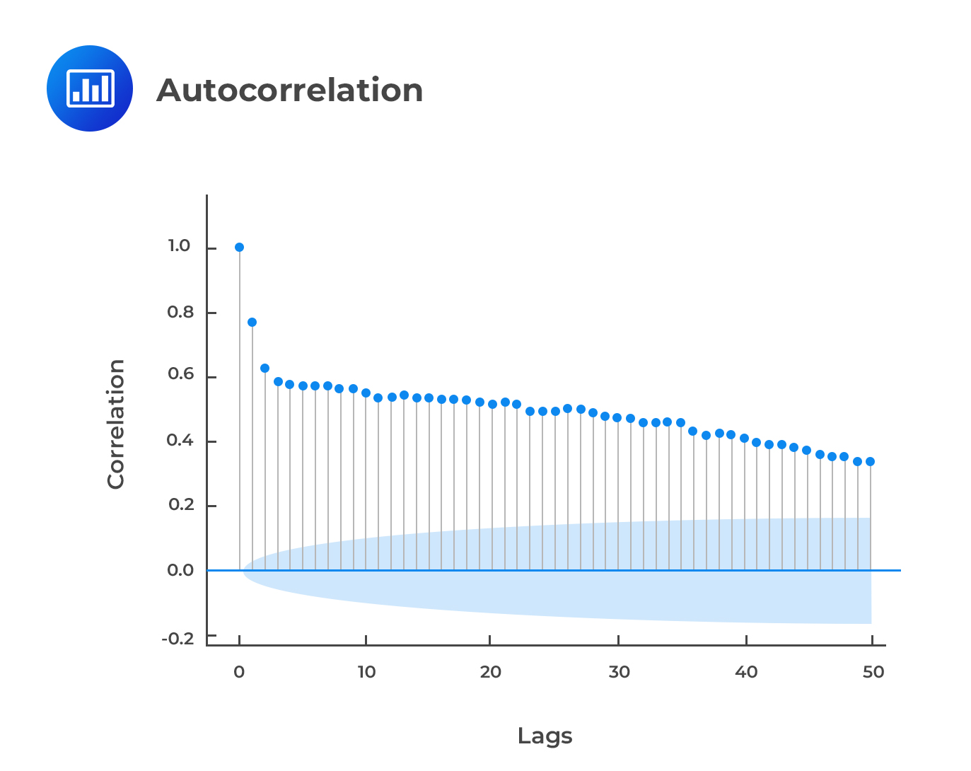
The Autcorrelation is defined as:

$$\rho\left(t\right)=\frac{Cov(Y_{t},Y_{t_h})}{\sqrt{V(Y_t) \sqrt{V(Y_{t-h})}}}=\frac{{\gamma}_{h}}{\sqrt{{\gamma}_{0}{\gamma}_{0}}}=\frac{{\gamma}_{h}}{{\gamma}_{0}}$$

Similarly, for \(h=0\).

$$\rho\left(t\right)=\frac{{\gamma}_{0}}{{\gamma}_{0}}=1$$

The autocorrelation ranges from -1 and 1 inclusively. The partial autocorrelation function is denoted as, \(p(h)\), and in a linear population regression of \(Y_t\) on \(Y_{t-1},…,Y_{t-h}\), it is the coefficient of \(y_{t-h}\). This regression is referred to as the autoregression. This is because the regression is on the lagged values of the variable.

White Noise

Assume that:

$$ { y }_{ t }={ \epsilon }_{ t } $$

$$ { \epsilon }_{ t }\sim \left( 0,{ \sigma }^{ 2 } \right) ,\quad \forall \quad { \sigma }^{ 2 }<\infty $$

where \({ \epsilon }_{ t }\) is the shock and is uncorrelated over time. Therefore, \({ \epsilon }_{ t }\) and \({ y }_{ t }\) are said to be serially uncorrelated.

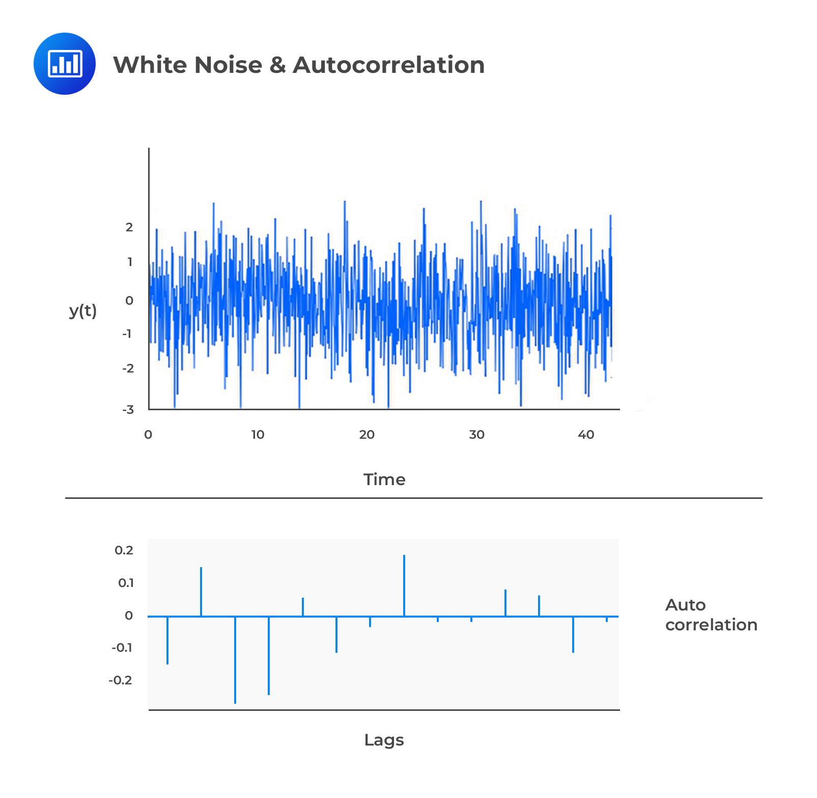This auto-correlation that has a zero mean and unchanging variance is referred to as the zero-mean white noise (or just white noise) and is written as:

$$ { \epsilon }_{ t }\sim WN\left( 0,{ \sigma }^{ 2 } \right) $$

And:

$$ { y }_{ t }\sim WN\left( 0,{ \sigma }^{ 2 } \right) $$

\({ \epsilon }_{ t }\) and \({ y }_{ t }\) serially uncorrelated but not necessarily serially independent. If \(y\) possesses this property, (serially uncorrelated but not necessarily serially independent) then it is said to be an independent white noise.

Therefore, we write:

$$ { y }_{ t }\underset { \sim }{ iid } \left( 0,{ \sigma }^{ 2 } \right) $$

This is read as “\(y\) is independently and identically distributed with a mean 0 and constant variance. \(y\) is said to be serially independent if it is serially uncorrelated and it has a normal distribution. In this case, \(y\) is called the normal white noise or the Gaussian white noise.

Written as:

$$ { y }_{ t }\underset { \sim }{ iid } N\left( 0,{ \sigma }^{ 2 } \right) $$

To characterize the dynamic stochastic structure of \({ y }_{ t }\sim WN\left( 0,{ \sigma }^{ 2 } \right) \), it follows that the unconditional mean and variance of \(y\) are:

$$ E\left( { y }_{ t } \right) =0 $$

And:

$$ var\left( { y }_{ t } \right) ={ \sigma }^{ 2 } $$

These two are constant since only displacement affects the autocovariances rather than time. All the autocovariances and autocorrelations are zero beyond displacement zero since white noise is uncorrelated over time.

The following is the autocovariance function for a white noise process:

$$ \gamma \left( h \right) =\begin{cases} { \sigma }^{ 2 },\quad h =0 \\ 0,\quad \quad h \ge 0\quad \quad \end{cases} $$

The following is the autocorrelation function for a white noise process:

$$ \rho \left( h \right) =\begin{cases} 1,\quad \quad h =0 \\ 0,\quad \quad h \ge 1\quad \end{cases} $$

Beyond displacement zero, all partial autocorrelations for a white noise process are zero. Thus, by construction white noise is serially uncorrelated. The following is the function of the partial autocorrelation for a white noise process:

$$ p\left( h \right) =\begin{cases} 1,\quad \quad h =0 \\ 0,\quad \quad h \ge 1\quad \end{cases} $$

Simple transformations of white noise are considered in the construction of processes with much richer dynamics. Then the white noise should be the 1-step-ahead forecast errors from good models.

The mean and variance of a process, conditional on its past, is another crucial characterization of dynamics with crucial implications for forecasting.

To compare the conditional and unconditional means and variances, consider the independence white noise: \({ y }_{ t }\underset { \sim }{ iid } \left( 0,{ \sigma }^{ 2 } \right) \). \(y\) has an unconditional mean and variance of zero and \({ \sigma }^{ 2 }\) respectively. Now, consider the transformational set:

$$ { \Omega }_{ t-1 }=\left\{ { y }_{ t-1 },{ y }_{ t-2 },\dots \right\} $$

Or:

$$ { \Omega }_{ t-1 }=\left\{ { \epsilon }_{ t-1 },{ \epsilon }_{ t-2 },\dots \right\} $$

The conditional mean and variance do not necessarily have to be constant. The conditional mean for the independent white noise process is:

$$ E\left( { y }_{ t }|{ \Omega }_{ t-1 } \right) =0 $$

The conditional variance is:

$$ var\left( { y }_{ t }|{ \Omega }_{ t-1 } \right) =E\left( { \left( { y }_{ t }-E\left( { y }_{ t }|{ \Omega }_{ t-1 } \right) \right) }^{ 2 }|{ \Omega }_{ t-1 } \right) ={ \sigma }^{ 2 } $$

Independent white noise series have identical conditional and unconditional means and variances.

Wold’s Theorem

Assuming that \(\left\{ { y }_{ t } \right\} \) is any zero-mean covariance-stationary process. Then:

$$ { Y }_{ t }=ϵ_t+β_{1} ϵ_{t-1} +β_{2} ϵ_{t-2}+\dots=\sum _{ i=0 }^{ \infty }{ { \beta }_{ i }{ \epsilon }_{ t-i } } $$

Where:

$$ { \epsilon }_{ t }\sim WN\left( 0,{ \sigma }^{ 2 } \right) $$

Note that \({ \beta }_{ 0 }=1\) and \(\sum_{ i=0 }^{ \infty }{{\beta}_{ i }^{ 2 }}<\infty\).

The accurate model for any stationary covariance series is the Wold’s representation. Since \({ \epsilon }_{ t }\) corresponds to the 1-step-ahead forecast errors to be incurred should a particularly good forecast be applied, the \({ \epsilon }_{ t }\)’s are the innovations.

Time-Series Models

The Autoregressive (AR) Models

AR models are time series models mostly used in finance and economics which links the stochastic process \(Y_t\) to the previous value \(Y_{t-1}\). The first order AR model denoted by AR(1) is given by:

$$Y_t=α+βY_{t-1}+ϵ_t$$

Where:

\(α\) = intercept

\(β\) = AR parameter

\(ϵ_t\) = the shock which is white noise \((ϵ_{t}\sim WN\left(0,σ^2\right)\)

Since\({Y_t}\) is assumed to be covariance stationary, the mean,variance, and autocovariances are all constant. By the principle of covariance stationarity,

$$E(Y_{t}) =E(Y_{t-1})=μ$$

Therefore,

$$E(Y_{t})=E(α+βY_{t-1}+ϵ_{t} =α+βE(Y_{t-1})+E(ϵ_{t})$$

$$\Rightarrow \mu =\alpha +\beta \mu +0 $$

$$\therefore \mu =\frac{\alpha}{1-\beta}$$

And for the variance,

$$V \left(Y_{t}\right)=V\left(α+βY_{t-1}+ϵ_{t}\right)=β^{2} V(Y_{t-1} )+V(ϵ_{t})+Cov(Y_{t-1},ϵ_{t})$$

$$γ_{0}=β^{2} γ_{0}+σ^{2}+0$$

$$\therefore \frac{{\sigma}^2}{1-{\beta}^2}$$

Note that \(Cov(Y_{t-1},ϵ_{t})\)=0 since \(Y_{t-1}\) is uncorrelated with the shocks \(ϵ_{t-1},ϵ_{t-2},…\)

The Autocovariances for AR(1) process is calculated recursively. The first autocovariance for the AR(1) model is given by:

$$ \begin{align*} Cov(Y_t,Y_{t-1} )&=Cov(α+βY_{t-1}+ϵ_t,Y_{t-1})\\ & =βCov(Y_{t},Y_{t-1} )+Cov(Y_{t-1},ϵ_{t}) \\ & =βγ_{0} \\ \end{align*} $$

The remaining autocovariance is recursively calculated as:

$$ \begin{align*} Cov(Y_t,Y_{t-h}) )&=Cov(α+βY_{t-1}+ϵ_{t},Y_{t-h})\\ & =βCov(Y_{t-1},Y_{t-h} )+Cov(Y_{t-h},ϵ_{t}) \\ & =β{\gamma}_{h-1} \\ \end{align*} $$

It should be easy to see that \(Cov(Y_{t-h},ϵ_{t} )=0\). Applying this recursion analogy:

$$γ_{h}=β^{h} {\gamma}_{0}$$

Therefore we can generalize the autocovariance as:

$$γ_{h}=β^{|h|} {\gamma}_{0}$$

Intuitively the autocorrelation function is given by:

$$\rho\left(\rho\right)=\frac{{\beta}^{h}{\gamma}_{0}}{{\gamma}_{0}}={\beta}^{|h|}$$

The ACF tends to 0 when h increases and that -1<β<0. The Partial autocorrelation of an AR(1) model is given by:

$$\partial \left(h\right)=\begin{cases}&{\beta}^{|h|},h \in \{0,±\}\\ &0, h≥2 \end{cases}$$

The Lag Operator

The lag operator denoted by L is important for manipulating complex time-series models. As its name suggests, the lag operator moves the index of a particular observation one step back. That is:

$$LY_{t}=Y_{t-1}$$

Properties of the Lag Operator

(I). The lag operator moves the index of a time series one step back. That is:
$$LY_{t}=Y_{t-1}$$

(II). Consider the following mth-order lag operator polynomial Lm then:

$$L^{m} Y_{t}=y_{t-m}$$For instance \(L^{2} Y_{t}=L(LY_{t} )=L(Y_{t-1} )=Y_{t-2}\)

(III). The lag operator of a constant is just a constant.

For example \(Lα=α\)

(IV). The p^th order lag operator is given by:

$$a(L)=1+a_{1} L+a_{2} L^{2}+…+a_{p} L^{p}$$

so that:

$$a(L) Y_{t}=Y_{t}+a_{1} Y_{t-1}+a_{2} Y_{t-2}+…+a_{p} Y_{t-p}$$

(V). The lag operator has a multiplicative property. Consider two lag operators a(L) and b(L). Then:

$$ \begin{align*} a(L)b(L)Y_t&=\left(1+a_{1} (L)\right)\left(1+b_{1} (L)\right)Y_t \\ & =\left(1+ a_{1} (L)\right)\left(Y_{t}+b_{1} Y_{t-1}\right)\\ & =Y_{t}+b_{1} Y_{t-1}+a_{1} Y_{t-1}+a_{1} b_{1} Y_{t-2} \\ \end{align*} $$

Moreover, the lag operator has a commutative property so that:

$$a(L)b(L)=b(L)a(L)$$

IV. Under some restrictive conditions, the lag operator polynomial can be inverted so that: \(a(L)a(L)^{-1}\)=1. When a(L) is a first-order lag operator polynomial given by \(1-a_{1} (L)\), is invertible if \(|a_{1} |<1\) so that its inverse is given by:

$$\left(1-a_{1}(L)\right)^{-1}=\sum _{i=1}^{\infty}{a^{i}L^{i}}$$

For an AR(1) model,

$$Y_{t}=α+βY_{t-1}+ϵ_{t}$$

This can be expressed with the lag operator so that:

$$Y_{t}=α+β(LY)_{t}+ϵ_{t}$$

$$⇒(1-βL) Y_{t}=α+ϵ_{t}$$

If |β|<1, then the lag polynomial above is invertible so that:

$$(1-βL)^{-1} (1-βL) Y_{t}=(1-βL)^{-1} α+(1-βL)^{-1} ϵ_{t}$$

$$\Rightarrow Y_{t}=\alpha \sum _{i=1}^{\infty}{{\beta}^{i}}+\sum _{j=1}^{\infty}{{\beta}^{j}L^{j}{\epsilon}_{t}}=\frac{\alpha}{1-\beta}+\sum _{i=1}^{\infty}{{\beta}^{i}L^{i}{\epsilon}_{t-i}}$$

The p^th Order Autoregressive Model (AR(p))

The AR(p) model is a generalization of the AR(1) model to include the p lags of \(Y_{t-1}\). Thus, the AR(p) is given by:

$$Y_{t}=α+β_{1} Y_{t-1}+β_{2} Y_{t-1}+…+β_{p} Y_{t-p}+ϵ_{t}$$

If \(Y_t\) is covariance stationary, then the long-run mean is given by:

$$E\left(Y_{t}\right)=\frac{\alpha}{1-{\beta}_{1}-{\beta}_{2}-\dots {\beta}_{p}}$$

And the long-run variance is given by:

$$V\left(Y_{t}\right)={\gamma}_{0}=\frac{\sigma^2}{1-{\beta}_{1}{\rho}_{1}-{\beta}_{2}{\rho}_{2}-\dots {\beta}_{p}{\rho}_{p}}$$

From the formulas of the mean and variance of the AR(p) model, the covariance stationarity property is satisfied if:

$$β_{1}+β_{2}+\dots +β_{p}<1$$

Otherwise, the covariance stationarity will be violated.

The autocorrelations function of the AR(p) model bears the same structural model as AR(1) model; the ACF tends to 1 as the length between the two-time series increases and may oscillate. However, higher-order ARs may bear complex structures in their ACFs.

The Moving Average Models (MA)

The first-order moving average model denoted by MA(1) is given by:

$$Y_{t}=μ+θϵ_{t-1}+ϵ_{t}$$

Where \(ϵ_{t} \sim WN(0,σ^{2})\).

Evidently, the process \(Y_t\) depends on the current shock \(ϵ_t\) and the previous shock \(ϵ_{t-1}\) where the coefficient θ measures the magnitude at which the previous shock affects the process. Note \(μ\) is the mean of the process since:

$$ \begin{align*} E(Y_{t} )&=E(μ+θϵ_{t-1}+ϵ_{t})=E(μ)+θE(ϵ_{t-1} )+E(ϵ_{t})\\ & =μ+0+0=μ \\ \end{align*} $$

For \(θ>0\), MA(1) is persistent because the consecutive values are positively correlated. On the other hand, if \(θ<0\), the process mean reverts because the effect of the previous shock is reversed in the current period.

The MA(1) model is always a covariance stationary process. The mean is as shown above, while the variance of the MA(1) model is given by:

$$ \begin{align*} V(Y_{t})&=V(μ+θϵ_{t-1}+ϵ_{t} )=V(μ)+θ^{2} V(ϵ_{t-1} )+V(ϵ_{t})\\ & =0+θ^{2} V(ϵ_{t-1} )+V(ϵ_{t} )=θ^{2} σ^{2}+σ^{2} \\ ⇒V(Y_{t} )&=σ^{2} (1+θ^{2}) \\ \end{align*} $$

The variance uses the intuition that the shock is white noise processes that are uncorrelated.

The MA(1) model has a non-zero autocorrelation function given by:

$$\rho\left(h\right)=\begin{cases}&1, h =0\\ & \frac{\theta}{1+{\theta}^{2}},h =1\\&0,h ≥2\end{cases}$$

The partial autocorrelations (PACF) of the MA(1) model is a complex and non-zero at all lags.

From the MA(1), we can generalize the q^th order MA process. Denoted by MA(q), it is given by:

$$Y_{t}=μ+ϵ_{t}+θ_{1 ϵ_{t-1}}+…+θ_q ϵ_{t-q}$$

The mean of the MA(q) process is still \(μ\) since all the shocks are white noise process (their expectations are 0). The autocovariance function of the MA(q) process is given by:

$$\gamma \left(h\right)=\begin{cases}&{\sigma}^{2}\sum_{i=0}^{q-h}{{\theta}_{i}{\theta}_{i+h}},0≤h≤q\\ & 0, h >q \end{cases}$$

And \(θ_0\)=1

The value of \(\theta\) can be determined by substituting the value taken by the autocorrelation function and solving the resulting quadratic equation. The partial autocorrelation of an MA(q) model is complex and non-zero at all lags.

Example: Moving Average Process.

Given an MA(2), \(Y_{t}=3.0+5ϵ_{t-1}+5.75ϵ_{t-2}+ϵ_{t}\) where \(ϵ_{t}\sim WN (0,σ^{2})\). What is the mean of the process?

Solution

The MA(2) is given by:

$$Y_{t}=μ+θ_{1} ϵ_{t-1}+θ_{2} ϵ_{t-2}+ϵ_{t}$$

Where μ is the mean. So, the mean of the above process is 3.0

The Autoregressive Moving Average (ARMA) Models

The ARMA model is a combination of AR and MA processes. Consider a first-order ARMA model (ARMA(1,1)). It is given by:

$$Y_{t}=α+βY_{t-1}+θϵ_{t-1}+ϵ_{t}$$

The mean of the ARMA(1,1) model is given by:

$$\mu = \frac{\alpha}{1-\beta}$$

And variance is given by

$${\gamma}_{0}=\frac{{\sigma}^{2}\left(1+2\beta \theta \right)}{1-{\beta}^2}$$

The autocovariance function is given by:

$$\gamma\left(h\right)=\begin{cases}&{\sigma}^{2}\frac{1+2\beta\theta +{\theta}^{2}}{1-{\beta}^{2}},h =0\\ &{\sigma}^{2}\frac{β(1+βθ)+θ(1+βθ)}{1-{\beta}^{2}},h=1\\ &\beta{\gamma}_{h-1},h ≥2 \end{cases}$$

The ACF form of the ARMA(1,1) decays as the length h increases and oscillate if \(β<0\), which is consistent with the AR model.

The PACF tends to 0 as the length h increase, which is consistent with the MA process. The decay of ARMA’s ACF and PACF is slow, which distinguishes it from the pure AR and MA models.

From the variance formula of ARMA(1,1), it is easy to see that the process is covariance stationery if \(|β|<1\)

ARMA(p,q) Model

As the name suggests, ARMA(p,q) is a combination of the AR(p) and MA(q) process. Its form is given by:

$$Y_{t}=α+β_{1} Y_{t-1}+…+β_{p} Y_{t-p}+θϵ_{t-1}+…+θ_{q} ϵ_{t-q}+ϵ_{t}$$

When expressed using lag polynomial, this expression reduces to:

$$β(L) Y_{t}=α+θ(L) ϵ_{t}$$

Analogous to ARMA(1,1), ARMA(p,q) is covariance -stationary if the AR portion is covariance stationary. The autocovariance and ACFs of the ARMA process are complex that decay at a slow pace to 0 as the lag \(h\) increases and possibly oscillate.

Sample Autocorrelation

The sample autocorrelation is utilized in validating the ARMA models. The autocovariance estimator is given by:

$$\hat{\gamma}_{h}=\frac{1}{T-h}\sum_{i=h +i}^{T}{\left(Y_{i} -\bar{Y}\right)\left(Y_{i-h}-\bar{Y}\right)}$$

Where \(\bar{Y}\) is the full sample mean.

The autocorrelation estimator is given by:

$$\hat{\rho}_{h}=\frac{\sum _{i=h +i}^{T}{\left(Y_{i} -\bar{Y}\right)\left(Y_{i-h}-\bar{Y}\right)}}{\sum_{i=1}^{T}{\left(Y_{i}-\bar{Y}\right)^{2}}}=\frac{\hat{\gamma}_{h}}{\hat{\gamma}_{0}}$$

The autocorrelation is such that \(-1≤\hat{\rho}≤1\)

Test for Autocorrelation

Test for autocorrelation is done using the graphical examination by plotting ACF and PACF of the residuals and check for any deficiencies such as inadequacy of the model to capture the dynamics of the data. However, graphical methods are unreliable.

The common tests used are Box-Pierce and Ljung-Box tests.

Box-Pierce and Ljung-Box Tests.

Box-Pierce and Ljung-Box test both tests the null hypothesis that:

$$H_{0}:ρ_{1}=ρ_{2}=…=ρ_{h}=0$$

Against the alternative that:

$$H_{1}:ρ_{j}≠0 (\text{At least one is non-zero})$$

Both the test are chi-distributed (\({\chi}_{h}^{2}\)) random variables. If the test statistic is larger than the critical value, the null hypothesis is rejected.

Box-Pierce Test

The test statistic under the Box-Pierce is given by:

$$Q_{BP}=T\sum _{i=1}^{h}{\hat{\rho}_{i}^{2}}$$

That is, the test statistic is the sum of squared autocorrelation scaled by the sample size T, which is (\({\chi}_{h}^{2}\)) random variable if the null hypothesis is true.

Ljung-Box Test

Ljung-Box test is a revised version of Box-Pierce that is appropriate with small sample sizes. The test statistic is given by:

$$Q_{LP}=T\left(T+2\right)\sum_{i=1}^{h}{\left(\frac{1}{T-i}\right)\hat{\rho}_{i}^{2}}$$

The Ljung-Box test statistic is also \({\chi}_{h}^{2}\) random variable.

Model Selection

The first step in model selection is the inspection of the sample autocorrelations and the PACFs. This provides the initial signs of the correlation of the data and thus can be used to select the type of models to be used.

The next step is to measure the fit of the selected model. The most commonly used method of measuring the model’s fit is Mean Squared Error (MSE) which is defined as:

$$\hat{\sigma}^{2}=\frac{1}{T}\sum_{t=1}^{T}{\hat{\epsilon}_{t}^{2}}$$

When the MSE is small, the model selected explains more of the time series. However, choosing a model with a small MSE implies that we need to increase the coefficient of variation R², which can lead to overfitting. To attend to this problem, other methods have been developed to measure the fit of the model. These methods involve adding an adjustment factor to MSE each time a parameter is added. These measures are termed as the Information Criteria (IC). There are two such ICs: Akaike Information Criteria (AIC) and the Bayesian Information Criteria (BIC).

Akaike Information Criteria (AIC)

Akaike Information Criteria (AIC) is defined as:

$$AIC=\text{T ln} \hat{\sigma}^2+2k$$

Where T is the sample size, and k is the number of the parameter. The AIC model adds the adjustment of adding two more parameters.

Bayesian Information Criteria (BIC).

Bayesian Information Criteria (BIC) is defined as:

$$BIC=\text{T ln} \hat{\sigma}^{2}+k ln T$$

Where the variables are defined as in AIC; however, note that the adjustment factor in BIC increases with an increase in the sample size T. Hence, it is a consistent model selection criterion. Moreover, the BIC criterion does not select the model that is larger than that selected by AIC.

The Box-Jenkin Methodology

The Box-Jenkin methodology provides a criterion of selecting between models that are equivalent but with different parameter values. The equivalency of the models implies that their mean, ACF and PACF are equal.

The Box-Jenkin methodology postulates two principles of selecting the models. One of the principles is termed as Parsimony. Under this principle, given two equivalent models, choose a model with fewer parameters.

The last principle is invertibility, which states that when selecting an MA or ARMA, select the model such that the coefficient in MA is invertible.

Model Forecasting

Forecasting is the process of using current information to forecast the future. In time series forecasting, we can make a one-step forecast or any time horizon h.

The one-step forecast time series forecasts the conditions expectation \(E(Y_{T+1} |Ω_{T})\). \(Ω_{T}\) is termed as the information set at time T which includes the entire history of Y (Y_T, Y_T-1…) and the shock history (\(ϵ_{T},ϵ_{T-1}…\)). In practice, this forecast is shortened to \(E_{T} \left(Y_{T+1}\right)\) so that:

$$E_{T} \left(Y_{T+1}│Ω_{T}\right)=E_{T}\left(Y_{T+1}\right)$$

Principles of Forecasting.

There are three rules of forecasting:

I. The expectation of a variable is the realization of that variable. That is: \(E_{T} \left(Y_{T}\right)=Y_{T}\). This applies to the residuals: \(E_{T} \left(ϵ_{T-1}\right)=ϵ_{T-1}\)

II. The value of the expectation of future shocks is always 0. That is,

$$E_{T} (ϵ_{T+h} )=0$$

III. The forecasts are done recursively, beginning with \(E_{T}(Y_{T+1})\) and that the forecast of a given time horizon might depend on the forecast of the previous horizon.

Let us consider some examples.

For the AR(1) model, the one-step forecast is given by:

$$ \begin{align*} E_{T} \left(Y_{T+1}\right) &=E_{T} \left(α+βY_{T}+ϵ_{T+1}\right)=α+βE_{T} (Y_{T} )+0\\ & =α+βY_{T} \\ \end{align*} $$

Note that we are using the current values \(Y_{T}\) to predict \(Y_{T+1}\) and shock used is that of the future \(ϵ_{T+1}\).

The two-step forecast is given by:

$$ \begin{align*} E_{T} \left(Y_{T+2}\right) & =E_{T}\left(α+βY_{T+1}+ϵ_{T+2}\right)\\ & =α+βE_{T} \left(Y_{T+1}\right)+E_{T}\left(ϵ_{T+2}\right) \\ \end{align*} $$

But \(E_{T} \left(ϵ_{T+2}\right)=0\) and \(E_{T} \left(Y_{T+1}\right)=α+βY_{T}\)

So that:

$$ \begin{align*} E_{T} \left(Y_{T+2}\right)&=α+βE_{T}\left(α+βY_{T}\right)=α+β\left(α+βY_{T}\right)\\ ⇒E_{T}\left(Y_{T+2}\right)&=α+αβ+β^{2} Y_{T} \\ \end{align*} $$

Analogously, the forecast for time horizon \(h\) we have:

$$ \begin{align*} E_{T} \left(Y_{T+h}\right)&=α+αβ+αβ^{2}+…+αβ^{h-1}+β^{h} Y_{T}\\ & = \sum_{i=1}^{h}{\alpha {\beta}^{i}}+{\beta}^{h}Y_{T} \\ \end{align*} $$

The Mean Reverting Level

When \(h\) is large, \(β^{h}\) must be very small by the intuition of covariance stationary of \(Y_t\). Therefore, it can be shown that:

$$ \lim_{h \to \infty } \sum_{i=0}^{h}{\alpha {\beta}^{i}} {\beta}^{h}Y_{T}=\frac{\alpha}{1-\beta}$$

The limit is actually the mean of the AR(1) model. The mean-reverting level implies \(Y_{T}\) does not affect the future value of Y. That is,

$$\lim_{h \to \infty} E_{T}\left(Y_{T+h}\right)=E\left(Y_{t}\right)$$

The same procedure is applied to MA and ARMA models.

The forecast error is the difference between the true future value and the forecasted value, that is,

$$ϵ_{T+1}=Y_{T+1}-E_{T}\left(Y_{T+1}\right)$$

For longer time-horizon, the forecast is mostly functions of the model parameters.

Example: Model Forecasting

The ARMA(1,1) for modeling the default in premiums for an insurance company is given by

$$D_{t}=0.055+0.934D_{t-1}+ϵ_{t}$$

Given that \(D_{T}=1.50\), what is the first step forecast of the default?

Solution

We need:

$$ \begin{align*} E_{T} \left(Y_{T+1}\right) &=α+βY_{T}\\ ⇒E_{T}\left(D_{T+1}\right)&=0.055+0.934×1.5=1.4560 \\ \end{align*} $$

Seasonality of Time Series

Some time-series data are seasonal. For instance, the sales at the time of summer that may differ from that of winter. The time series with deterministic seasonality is termed as non-stationary, while those with stochastic seasonality are called stationary time series and hence modeled with AR or ARMA process.

A pure seasonal lag utilizes the lags at a seasonal frequency. For instance, assume that we are using the semi-annual data, then the pure seasonal AR(1) model of quarterly time seasonal time series is:

$$(1-βL^{4} )Y_{t}=α+ϵ_{t}$$

So that:

$$Y_{t}=α+βY_{t-4}+ϵ_{t}$$

A more efficient seasonality includes the short-term and seasonal lag components. The short-term components utilize the lags at the observation frequency.

Seasonality can also be introduced to AR, MA, or both models by multiplying the short run lag polynomial and by the seasonal lag polynomial. For instance, the seasonal ARMA is specified as:

$$ARMA \left(p,q)×(p_{s},q_{s}\right)_{f}$$

Where p and q are the orders of the short run-lag polynomials, and p_s and q_s are the seasonal lag polynomials. Practically, seasonal lag polynomials are restricted to one seasonal lag because the accuracy of the parameter approximations depends on the number of full seasonal cycles in the sample data.

Question 1

The following sample autocorrelation estimates are obtained using 300 data points:

$$\begin{array}{lccc} \textbf{Lag} & \textbf{1} & \textbf{2} & \textbf{3} \\ \textbf{Coefficient} & 0.25 & -0.1 & -0.05 \end{array}$$

Compute the value of the Box-Pierce Q-statistic.

1. 22.5
2. 22.74
3. 30
4. 30.1

The correct answer is A.

$$ \begin{align*} { Q }_{ BP }&=T\sum _{ h =1 }^{ m }{ { \hat { \rho } }^{ 2 } } \left( h \right)\\ & = 300({0.25}^{ 2 }+ {(-0.1)}^{2}+ {(-0.05)}^{2}) \\ &= 22.5 \\ \end{align*} $$

Question 2

The following sample autocorrelation estimates are obtained using 300 data points:

$$\begin{array}{lccc} \textbf{Lag} & \textbf{1} & \textbf{2} & \textbf{3} \\ \textbf{Coefficient} & 0.25 & -0.1 & -0.05 \end{array}$$

Compute the value of the Ljung-Box Q-statistic.

1. 30.1
2. 30
3. 22.5
4. 22.74

The correct answer is D.

$$ \begin{align*} { Q }_{ LB }&=T\left( T+2 \right) \sum _{ h =1 }^{ m }{ { \left( \widehat { \frac { 1 }{ T-h } } \right) } } { \rho }^{ 2 }\left( h \right) \\ &= 300(302)({ \frac {{0.25}^{ 2 }}{299}} + { \frac {{-0.1}^{ 2 }}{298}} + { \frac {{-0.05}^{ 2 }}{297}} ) \\ &= 22.74 \\ \end{align*} $$

Note: Provided the sample size is large, the Box-Pierce and the Ljung-Box tests typically arrive at the same result.

Question 3

Assume the shock in a time series is approximated by Gaussian white noise. Yesterday’s realization, y(t) was 0.015, and the lagged shock was -0.160. Today’s shock is 0.170.

If the weight parameter theta, θ, is equal to 0.70 and the mean of the process is 0.5, determine today’s realization under a first-order moving average, MA(1), process.

1. -4.205
2. 4.545
3. 0.558
4. 0.282

The correct answer is C.

Today’s shock = \({ \epsilon }_{ t }\); yesterday’s shock = \({ \epsilon }_{ t-1 }\); today’s realization = \({ y }_{ t }\); yesterday’s realization = \({ y }_{ t-1 }\).

The MA(1) is given by:

$$ \begin{align*} { y }_{ t }&= \mu +\theta { \epsilon }_{ t-1 }+{ \epsilon }_{ t } \\ &=0.5 + 0.170 + 0.7(-0.160) = 0.558\\ &= 0.558 \\ \end{align*} $$