Machine Learning Methods

After completing this reading, you should be able to:

• Discuss the philosophical and practical differences between machine learning techniques and classical econometrics.
• Compare and apply the two methods utilized for rescaling variables in data preparation.
• Explain the differences among the training, validation, and test data sub-samples, and how each is used.
• Understand the differences between and consequences of underfitting and overfitting, and propose potential remedies for each.
• Use principal components analysis to reduce the dimensionality of a set of features.
• Describe how the K-means algorithm separates a sample into clusters.
• Describe natural language processing and how it is used.
• Differentiate among unsupervised, supervised, and reinforcement learning models.
• Explain how reinforcement learning operates and how it is used in decision-making.

Machine-learning Techniques vs. Classical Econometrics

Machine learning (ML) is the art of programming computers to learn from data. Its basic idea is that systems can learn from data and recognize patterns without active human intervention. ML is best suited for certain applications, such as pattern recognition and complex problems that require large amounts of data and are not well solved with traditional approaches.

On the other hand, classical econometrics has traditionally been used in finance to identify patterns in data. It has a solid foundation in mathematical statistics, probability, and economic theory. In this case, the analyst researches the best model and the variables to use. The computer’s algorithm tests the significance of variables, and based on the results, the analyst decides whether the data supports the theory.

Machine learning and traditional linear econometric approaches are both employed in prediction. The former has several advantages: machine learning does not rely much on financial theory when selecting the most relevant features to include in a model. A researcher who is unsure or has not specified whether the relationship between variables is linear or non-linear can also use it. The ML algorithm automatically selects the most relevant features and determines the most appropriate relationships between the variables.

Secondly, ML algorithms are flexible and can handle complex relationships between variables. Consider the following linear regression model: $$y=\beta_0+\beta_1 X_1+\beta_2 X_2+\varepsilon$$

Assume that the effect of \(\mathrm{X}_1\) on \(\mathrm{y}\) depends on the level of \(\mathrm{X}_2\). Analysts would miss this interaction effect unless a multiplicative term was explicitly included in the model. In the case of many explanatory variables, a linear model may be difficult to construct for all combinations of interaction terms. The use of machine learning algorithms can mitigate this problem by automatically capturing interactions.

In addition, the traditional statistical approaches for evaluating models, such as analyses of statistical significance and goodness of fit tests, are not typically applied in the same way to supervised machine learning models. This is because the goal of supervised machine learning is often to make accurate predictions rather than to understand the underlying relationships between variables or to test hypotheses.

There are different terminologies and notations used in ML. This is because engineers, rather than statisticians, developed most machine learning techniques. There has been a lot of discussion of features/inputs and targets/outputs. According to classical econometrics, features/inputs are simply independent variables. Targets/outputs are dependent variables, and the values of the outputs are referred to as labels.

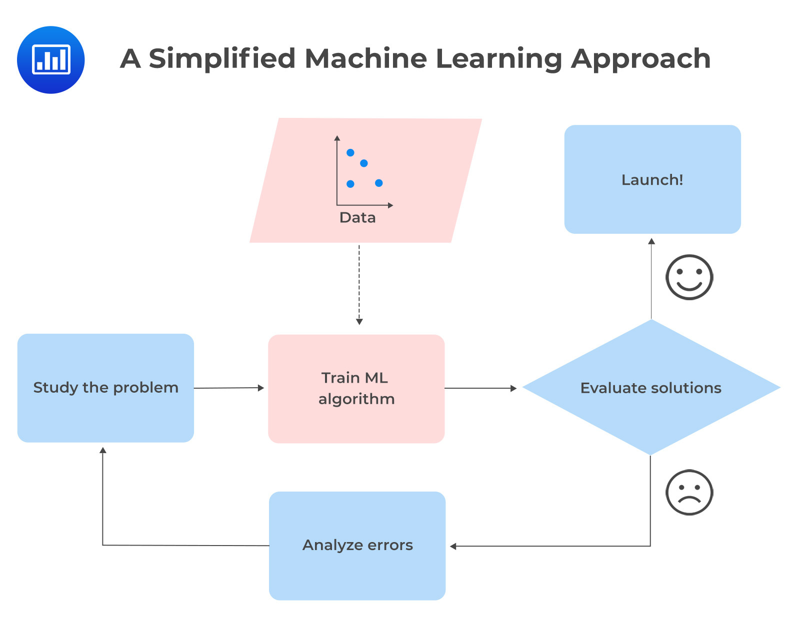The following gives a summary of some of the differences between \(\mathrm{ML}\) techniques and classical econometrics.

$$\small{\begin{array}{l|l|l}
&{ \textbf{Machine Learning}\\\textbf{Techniques}} & \textbf{Classical Econometrics} \\\hline
\text{Goals} & \begin{array}{@{\labelitemi\hspace{\dimexpr\labelsep+0.5\tabcolsep}}l@{}}\text{Builds models that can learn}\\\text{from data and continuously}\\\text{improve their performance}\\\text{with time, and do not need}\\\text{to specify the relationships}\\\text{between variables in advance.}\end{array} & \begin{array}{@{\labelitemi\hspace{\dimexpr\labelsep+0.5\tabcolsep}}l@{}}\text{Identifies and estimates the}\\\text{relationships between variables.}\\\text{It also tests the hypothesis}\\\text{about these relationships.}\end{array} \\\hline
{\text{Data}\\\text{requirements}} & \begin{array}{@{\labelitemi\hspace{\dimexpr\labelsep+0.5\tabcolsep}}l@{}}\text{ML models can deal with large}\\\text{amounts of complex and}\\\text{unstructured data.}\end{array} & \begin{array}{@{\labelitemi\hspace{\dimexpr\labelsep+0.5\tabcolsep}}l@{}}\text{Require well-structured}\\\text{and clearly defined}\\\text{dependent and independent}\\\text{variables.}\end{array} \\\hline
\text{Assumptions} & \begin{array}{@{\labelitemi\hspace{\dimexpr\labelsep+0.5\tabcolsep}}l@{}}\text{They are not built on} \\\text{assumptions and can handle} \\\text{non-linear relationships} \\\text{between variables.}\end{array} & \begin{array}{@{\labelitemi\hspace{\dimexpr\labelsep+0.5\tabcolsep}}l@{}}\text{Based on various assumptions, e.g.,}\\\text{errors are normally distributed,}\\\text{linear relationships}\\\text{between variables.}\end{array} \\\hline
\text{Interpretability} & \begin{array}{@{\labelitemi\hspace{\dimexpr\labelsep+0.5\tabcolsep}}l@{}}\text{Maybe complex to interpret,}\\\text{as they may involve complex}\\\text{patterns and relationships}\\\text{that are difficult to understand }\\\text{or explain.}\end{array} & \begin{array}{@{\labelitemi\hspace{\dimexpr\labelsep+0.5\tabcolsep}}l@{}}\text{Statistical models can}\\\text{be interpreted in terms}\\\text{of the relationships}\\\text{between variables.}\end{array} \end{array}}$$

Methods Utilized for Rescaling Variables in Data Preparation

Data Preparation

There is a tendency for ML algorithms to perform poorly when the variables have very different scales. For example, there is a vast difference in the range between income and age. A person’s income ranges in the thousands while their age ranges in the tens. Since ML algorithms only see numbers, they will assume that higher-ranging numbers (income in this case) are superior, which is false. It is, therefore, crucial to have values in the same range. Standardization and normalization are two methods for rescaling variables.

Standardization

Standardization involves centering and scaling variables. Centering is where the variable’s mean value is subtracted from all observations on that variable (so standardized values have a mean of 0). Scaling is where the centered values are divided by the standard deviation so that the distribution has a unit variance. This is expressed as follows:

$$ \mathrm{x}_{\mathrm{i} \text { (standardized) }}=\frac{\mathrm{x}_{\mathrm{i}}-\mu}{\sigma} $$

Normalization

Normalization, also known as min-max scaling, entails rescaling values from 0 to 1. This is done by subtracting the minimum value \(\left(\mathrm{x}_{\min }\right)\) from each observation and dividing by the difference between the maximum \(\left(\mathrm{x}_{\max }\right)\) and minimum values \(\left(\mathrm{x}_{\min }\right)\) of \(\mathrm{X}\). This is expressed as follows:

$$\mathrm{x}_{\mathrm{i} \text { (normalized })}=\frac{\mathrm{x}_{\mathrm{i}}-\mathrm{x}_{\min }}{\mathrm{x}_{\max }-\mathrm{x}_{\min } }$$

The preferable rescaling method depends on the data characteristics:

• Standardization is used when the data includes outliers. This is because normalization would compress data points into a narrow range of \(0-1\), which would be uncharacteristic of the original data.
• Data must be normally distributed for standardization to be used, whereas normalization can be used when the data distribution is unknown.

Data Cleaning

This is a crucial component of ML and may be the difference between an ML’s success and failure. Data cleaning is necessary for the following reasons:

• Missing data: Analysts encounter this issue very often. Missing data can be dealt with in the following ways. First, observations with only a small number of missing values can be removed. Secondly, they can replace them with the mean or median of the non-missing observations. Lastly, it may be possible to estimate the missing values based on observations of other features.
• Inconsistent recording: It is important to record data consistently so that it can be read correctly and easily used.
• Unwanted observations: Observations that are not relevant to the specific task should be removed. The result is a more efficient analysis and a reduction in distractions.
• Duplicate observations: Duplicate data points should be removed to avoid biases.
• Problematic features: A feature with many standard deviations from the mean should be carefully monitored as they can be problematic.

Training, Validation, Test Datasets

We briefly discussed the training and validation data sets, which are in-sample datasets. Additionally, there is an out-of-sample dataset, which is the test data. The training dataset teaches an ML model to make predictions, i.e., it learns the relationships between the input data and the desired output. A validation dataset is used to evaluate the performance of an ML model during the training process. It compares the performance of different models so as to determine which one generalizes (fits) best to new data. A test dataset is used to evaluate an ML model’s final performance and identify any remaining issues or biases in the model. The performance of a good ML model on the test dataset should be relatively similar to the performance on the training dataset. However, the training and test datasets may perform differently, and perfect generalization may not always be possible.

It is up to the researchers to decide how to subdivide the available data into the three samples. A common rule of thumb is to use two-thirds of the sample for training and the remaining third to be equally split between validation and testing. The subdivision of the data will be less crucial when the overall data points are large. Using a small training dataset can introduce biases into the parameter estimation because the model will not have enough data to learn the underlying patterns in the data accurately. Using a small validation dataset can lead to inaccurate model evaluation because the model may not have enough data to assess its performance accurately; thus, it will be hard to identify the best specification. When subdividing the data into training, validation, and test datasets, it is crucial to consider the type of data you are working with.

For cross-sectional data, it is best to divide the dataset randomly since the data has no natural ordering (i.e., the variables are not related to each other in any specific order). For time series data, it is best to divide the data into chronological order, starting with training data, then validation data, and testing data.

Cross-validation Searches

Cross-validation can be used when the overall dataset is insufficient to be divided into training, validation, and testing datasets. In cross-validation, training, and validation datasets are combined into one sample, and the testing dataset is excluded. The combined data is then equally split into sub-samples, with a different sub-sample left out each time as the test dataset. This technique is known as k-fold cross-validation. It splits the training and validation data into k sub-samples, and the model is trained and evaluated k times while leaving out the test data from the combined sample. The values k = 5 and k =10 are commonly chosen for k-fold cross-validation.

Overfitting and Underfitting

Understand the differences between and consequences of underfitting and overfitting, and propose potential remedies for each.

Overfitting

Imagine that you have traveled to a new country, and the shop assistant rips you off. It is a natural instinct to assume that all shop assistants in that country are thieves. If we are not careful, machines can also fall into the same trap of overgeneralizing. This is known as overfitting in ML.

Overfitting occurs when the model has been trained too well on the training data and performs poorly on new, unseen data. An overfitted model can have too many model parameters, thus learning the detail and noise in the training data rather than the underlying patterns. This is a problem because it means that the model cannot make reliable predictions about new data, which can lead to poor performance in real-world applications. The evaluation of the ML algorithm thus focuses on its prediction error on new data rather than on its goodness of fit on the trained data. If an algorithm is overfitted to the training data, it will have a low prediction error on the training data but a high prediction error on new data.

The dataset to which an ML model is applied is normally split into training and validation samples. The training data set is used to train the ML model by fitting the model parameters. On the other hand, the validation data set is used to evaluate the trained model and estimate how well the model will generalize into new data.

Overfitting is a severe problem in ML, which can easily have thousands of parameters, unlike classical econometric models that can only have a few parameters. Potential remedies for overfitting include decreasing the complexity of the model, reducing features, or using techniques such as regularization or early stopping.

Underfitting

Underfitting is the opposite of overfitting. It occurs when a model is too simple and thus not able to capture the underlying patterns in the training data. This results in poor performance on both the training data and new data. For example, we would expect a linear model of life satisfaction to be prone to underfit since the real world is more complicated than the model. In this scenario, the ML predictions are likely to be inaccurate, even on the training data.

Underfitting is more likely in conventional models because they tend to be less flexible than ML models. The former follows a predetermined set of rules or assumptions, while ML does not follow assumptions about the structure of the model. It should be noted, however, that ML models can still experience underfitting. This can happen when there is insufficient data to train the model, when the data is of poor quality, and if there is excessively stringent regularization.

Regularization is an approach commonly used to prevent overfitting. It adds a penalty to the model as the complexity model complexity increases. If the regularization is set too high, it can cause the model to underfit the data. Potential remedies for addressing underfitting include increasing the complexity of the model, adding more features, or increasing the amount of training data.

Bias-Variance Tradeoff

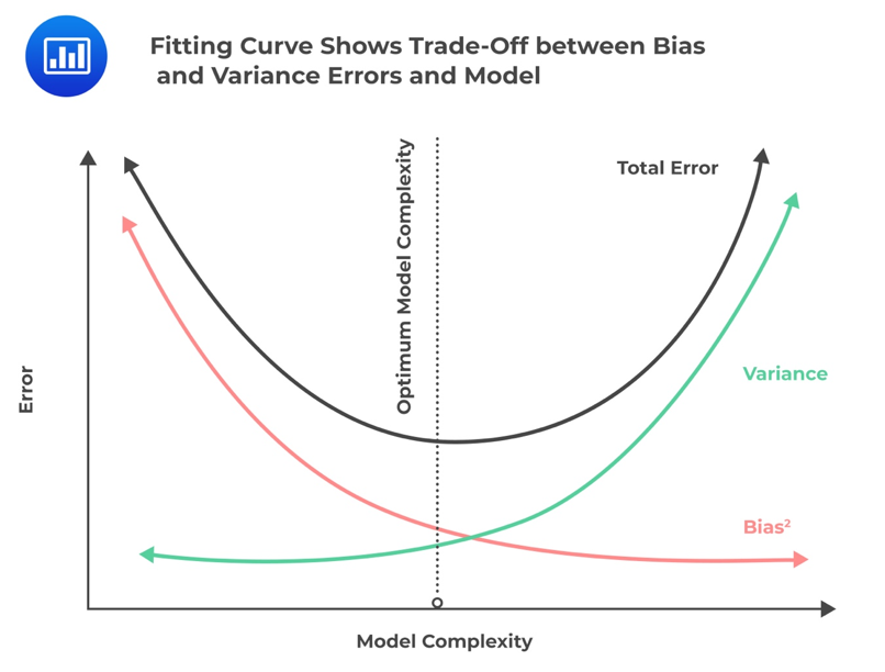
The complexity of the ML model, which determines whether the data is over, under, or well-fitted, involves a phenomenon called bias-variance tradeoff. Complexity refers to the number of features in a model and whether a model is linear or non-linear (with non-linear being too complex). Bias occurs when a complex model is approximated with a simpler model, i.e., by omitting relevant factors and interactions. A model with highly biased predictions is likely to be oversimplified and thus results in underfitting. Variance refers to how sensitive the model is to small fluctuations in the training data. A model with high variance in predictions is likely to be complex and thus results in overfitting.

The figure below illustrates how bias and variance are affected by model complexity.

Principal Components Analysis (PCA)

Training ML models can be slowed by the millions of features that might be present in each training instance. The many features can also make it difficult to find a good solution. This problem is referred to as the curse of dimensionality.

Dimensions and features are often used interchangeably. Dimension reduction involves reducing the features of a dataset without losing important information. It is useful in ML as it simplifies complex datasets, scales down the computational burden of dealing with large datasets, and improves the interpretability of models.

PCA is the most popular dimension reduction approach. It involves projecting the training dataset onto a lower-dimensional hyperplane. This is done by finding the directions in the dataset that capture the most variance and projecting the dataset onto those directions. PCA reduces the dimensionality of a dataset while preserving as much information as possible.

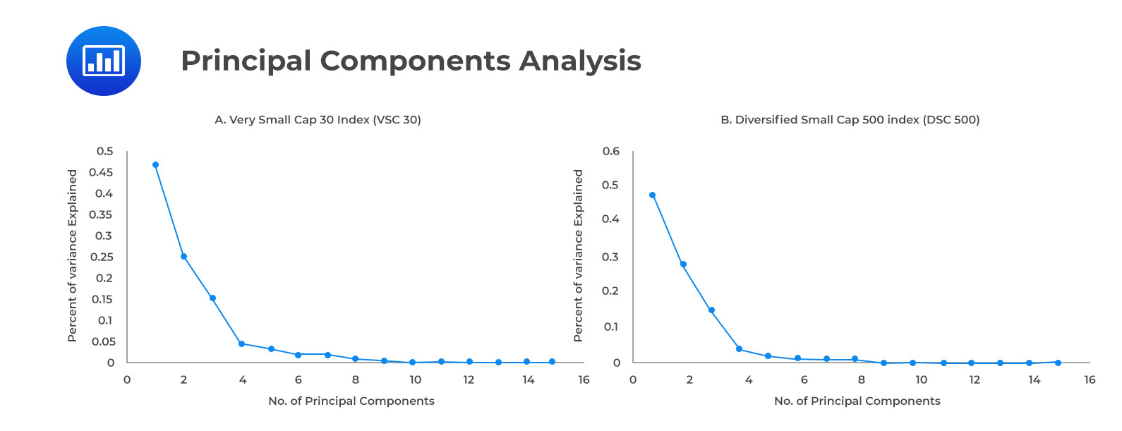
In PCA, the variance measures the amount of information. Hence, principal components capture the most variance and retain the most information. Accordingly, the first principal component will account for the largest possible variance; the second component will intuitively account for the second largest variance (provided that it is uncorrelated with the first principal component), and so on. A scree plot shows how much variance is explained by the principal components of the data. The principal components that explain a significant proportion of the variance are retained (usually 85% to 95%).

Example: Principal Components Analysis (PCA)

Researchers are concerned about which principal components will adequately explain returns in a hypothetical Very Small Cap (VSC) 30 and Diversified Small Cap (DSC) 500 equity index over a 15-year period. DSC 500 is a diversified index that contains stocks across all sectors, whereas VSC 30 is a concentrated index that contains technology stocks. In addition to index prices, the dataset contains more than 1000 technical and fundamental features. The fact that the dataset has so many features causes them to overlap due to multicollinearity. This is where PCA comes in handy, as it works by creating new variables that can explain most of the variance while preserving information in the data.

Below is a screen plot for each index. Based on the 20 principal components generated, the first three components explain 88% and 91% of the variance in the VSC 30 and DSC 500 index values, respectively. Screen plots for both indexes illustrate that the incremental contribution in explaining variance structure is very small after PC5 or so. From PC5 onwards, it is possible to ignore the principal components without losing important information.

The K-Means Clustering Algorithm

Clustering is a type of unsupervised machine-learning technique that organizes data points into similar groups. These groups are called clusters.

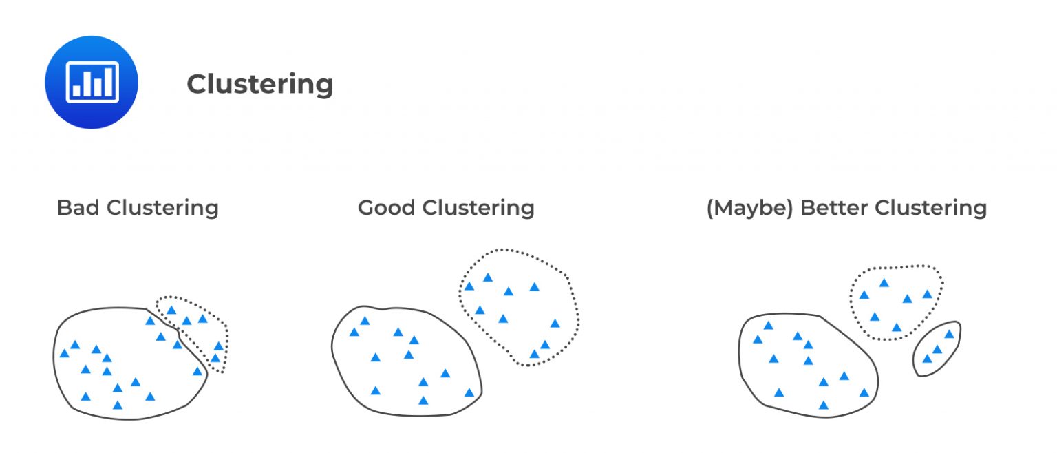
Clusters contain observations from data that are similar in nature. K-means is an iterative algorithm that is used to solve clustering problems. K is the number of fixed clusters the analyst determines at the outset. It is based on the idea of minimizing the sum of squared distances between data points and the centroid of the cluster to which they belong. Below is an outline of the process for implementing K-means clustering:

1. Randomly allocate initial K centroids within the data (centers of the clusters).
2. Assign each data point to the closest centroid, creating K clusters.
3. Calculate the new K centroids for each cluster by taking the average value of all data points assigned to that cluster.
4. Reassign each data point to the closest centroid based on the newly calculated centroids.
5. Repeat the process of recalculating the new K centroids until the centroids converge or a predetermined number of iterations has been reached.

Iterations continue until no data point is left to reassign to the closest centroid (there is no need to recalculate new centroids). The distance between each data point and the centroids can be measured in two ways. The first is the Euclidean distance, while the second is the Manhattan distance.

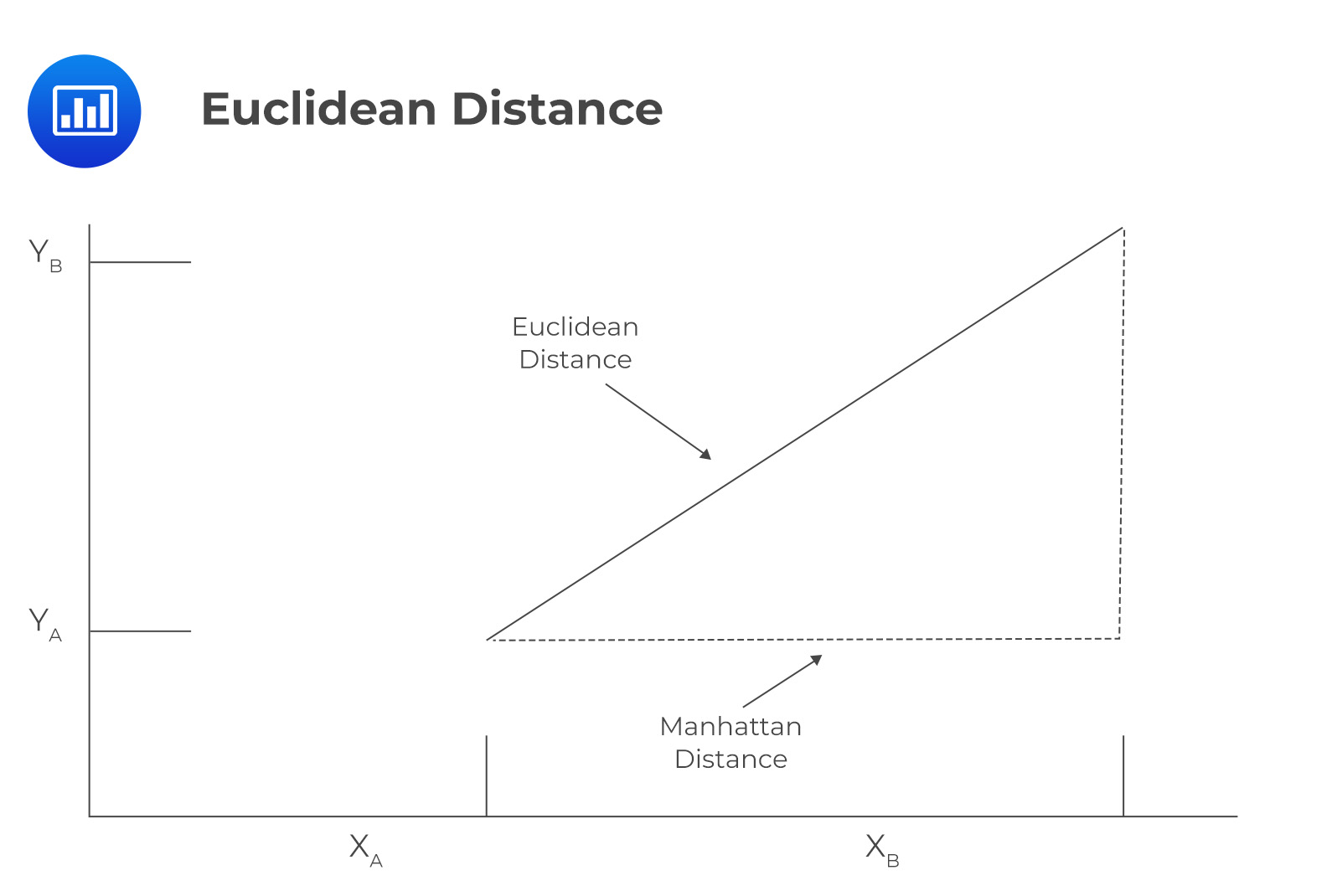Consider two features \(\mathrm{x}\) and \(\mathrm{y}\), which both have two data points \(\mathrm{A}\) and \(\mathrm{B}\), with coordinates \(\left(\mathrm{x}_{\mathrm{A}}, \mathrm{y}_{\mathrm{A}}\right)\) and \(\left(\mathrm{x}_{\mathrm{B}}, \mathrm{y}_{\mathrm{B}}\right)\), respectively. The Euclidean distance, also known as \(\mathrm{L}^2\) – norm, is calculated as the square root of the sum of the squares of the differences between the coordinates of the two points. Imagine the Pythagoras Theorem, where Euclidean distance is the unknown side of a right-angled triangle.

For a two-dimensional space, this is represented as:
$$ \text { Euclidean Distance }\left(d_E\right)=\sqrt{\left(x_B-x_A\right)^2+\left(y_B-y_A\right)^2} $$

In the case that there are more than two dimensions, for example, \(\mathrm{n}\) features for two data points \(\mathrm{A}\) and \(\mathrm{B}\), Euclidean distance will be constructed in a similar fashion. Euclidean distance is also known as the “straight-line distance ” because it is the shortest distance between two points, indicated by the solid line in the figure below. Manhattan distance, also known as \(L^1\) – norm, is calculated as the sum of the absolute differences between two coordinates. For a two-dimensional space, this is represented as:
$$ \text { Manhattan distance } \left(d_M\right)=\left|\mathrm{x}_{\mathrm{B}}-\mathrm{x}_{\mathrm{A}}\right|+\left|\mathrm{x}_{\mathrm{B}}-\mathrm{x}_{\mathrm{A}}\right| $$

Manhattan distance is named after the layout of streets in Manhattan, where streets are laid out in a grid pattern, and the only way to travel between two points is by going along the grid lines.

Example: Calculating Euclidean and Manhattan Distances

Suppose you have the following financial data for three companies:

Company P:

Feature 1: Market Capitalization = $0.5 billion.

Feature 2: P/E Ratio = 9.

Feature 3: Debt-to-Equity Ratio = 0.6.

Company Q:

Feature 1: Market Capitalization = $2.5 billion.

Feature 2: P/E Ratio = 15.

Feature 3: Debt-to-Equity Ratio = 8.

Company R

Feature 1: Market Capitalization = $85 billion.

Feature 2: P/E Ratio = 32.

Feature 3: Debt-to-Equity Ratio = 45.

Calculate the Euclidean and Manhattan distances between companies P and Q in feature space for the raw data.

Euclidean Distance

To calculate the Euclidean distance between companies P and Q in feature space for the raw data, we first need to find the difference between each feature value for the two companies and then square the differences. The Euclidean distance is then calculated by taking the square root of the sum of these squared differences.

$$\text{Euclidean Distance} \left(d_E\right)=\sqrt{(0.5-2.5)^2+(9-15)^2+(0.6-8)^2}=\sqrt{94.76}=9.73$$

Manhattan Distance

To calculate the Manhattan distance between companies \(P\) and \(Q\) in feature space for the raw data, we simply find the absolute difference between each feature value for the two companies and sum these differences. The Manhattan distance is then calculated by taking the sum of these differences. The Manhattan distance between companies \(P\) and \(Q\) in feature space is:

 $$\begin{align}\text{Manhattan Distance}\left(d_M\right)&=|0.5-2.5|+|9-15|+|0.6-8|=|-2|+|-6|+|-7.4|\\&=2+6+7.4=\$ 15.4\end{align}$$

Performance Measurement for K-means

Formulas described above indicate the distance between two points \(\mathrm{A}\) and \(\mathrm{B}\). Note that \(\mathrm{K}\)-means aims to minimize the distance between each data point and its centroid rather than to minimize the distance between data points. The data points will be closer to the centroids when the model fits better.

Inertia, also known as the Within-Cluster Sum of Squared errors (WCSS), is a measure of the sum of the squared distances between the data points within a cluster and the cluster’s centroid. Denoting the distance measure as \(\mathrm{d}_{\mathrm{i}}\), WCSS is expressed as:

$$\text{WCSS}=\sum_{i=1}^n d_i^2$$

The k-means algorithm aims to minimize the inertia by iteratively reassigning data points to different clusters and updating the cluster centroids until convergence. The final inertia value can be used to measure the quality of the clusters the K-means algorithm produces.

Choosing an Appropriate Value for K

Choosing an appropriate value for K can affect the performance of the K-means model. For example, if K is set too low, the clusters may be too general and may not be a true representative of the underlying structure of the data. Similarly, if K is set too high, the clusters may be too specific and may not represent the data’s overall structure. These clusters may not be useful for the intended purpose of the analysis in either case. It is, therefore, important to choose K optimally in practice.

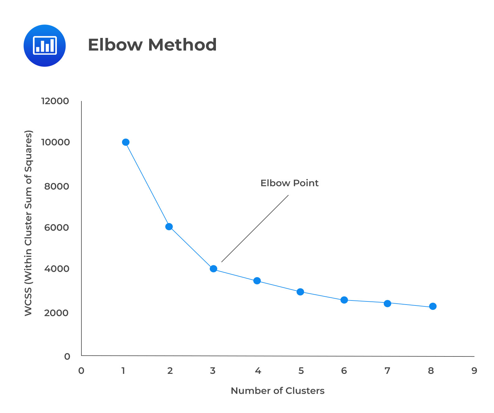
The optimal value of K can be calculated using different methods, such as the elbow method and the silhouette analysis. The elbow method fits the K-means model for different values of K and plots the inertia/ WCSS for each value of K. Similar to PCA, this is called a scree-plot. It is then examined for the obvious point on the plot where the inertia decreases more slowly as K increases (elbow), which is chosen as the optimal value of K. In other words, it is the value that corresponds to the “elbow” point in the scree plot.

The second approach involves fitting the K-means model for a range of values of K and determining the silhouette coefficient for each value of K. The silhouette coefficient compares the distance of each data point from other points in its own cluster with its distance from the data points in the other closest cluster. In other words, it measures the similarity of a data point to its own cluster compared to the other closest clusters. The optimal value of K is the one that corresponds to the highest silhouette coefficient across all data points.

Advantages and Disadvantages of the K-Means Algorithm

K-means clustering is simple and easy to implement, making it a popular choice for clustering tasks. There are some disadvantages to K-Means, such as the need to specify clusters, which can be difficult if the dataset is not well separated. Additionally, it assumes that the clusters are spherical and equal in size, which is not always the case in practice.

K-means algorithm is very common in investment practice. It can be used for data exploration in high-dimensional data to discover patterns and group similar observations together.

Natural Language Processing

Natural language processing (NLP) focuses on helping machines process and understand human language.

Steps Involved in NLP Process

The main steps in the NLP process are outlined below:

1. Data collection: Involves acquiring data from various sources, including financial statements, news articles, social media posts, etc.
2. Data preprocessing: The raw textual data is cleaned, formatted, and transformed into a form suitable for computer usage. Tasks such as tokenization, stemming, and stop word removal can be carried out at this stage.
3. Feature extraction: This involves extracting relevant features from the preprocessed data. It may involve extracting financial metrics, sentiments, and other relevant information.
4. Model training: This involves training the machine learning model using the extracted features.
5. Model evaluation: This involves evaluating the performance of the trained model to ensure it generates accurate and reliable predictions. Techniques such as cross-validation can be employed here. Model evaluation is carried out on the test dataset.
6. Model deployment: The evaluated model is then deployed for use in real-world investment scenarios.

Data Preprocessing

Textual data (unstructured data) is more suitable for human consumption rather than for computer processing. Unstructured data thus needs to be converted to structured data through cleaning and preprocessing, a process called text processing. Text cleansing involves involving removing HTML tags, punctuations, numbers, and white spaces (e.g., tabs and indents).

The next step is text wrangling (preprocessing) which involves the following:

1. Tokenization: Involves separating a piece of text into smaller units called tokens. It allows the NLP model to analyze the textual data more easily by breaking it down into individual units that can be more easily processed.
2. Lowercasing: To avoid discriminating between “stock” and “Stock.”
3. Removing stop words: These are words with no informational value, e.g., as, the, and is, used as sentence connectors. They are eliminated to reduce the number of tokens in the training data.
4. Stemming: Reduces all the variations of a word into a common value (base form/stem): For example, “earned,” “earnings,” and “earning.” are all assigned a common value of earn. It only removes the suffixes of words.
5. Lemmatization: Involves reducing words to their base form/lemma to identify related words. Unlike stemming, lemmatization incorporates the full structure of the word and uses a dictionary or morphological analysis to identify the lemma. It generates more accurate base forms of words. However, it is more computationally expensive compared to stemming.
6. Consider “n-grams:” These are words that need to be placed together to give a specific meaning. For example, “strong earnings,” “negative outlook,” or “market uncertainty.”

Finance professionals can leverage on NLP to derive insights from large chunks of data to make more informed decisions. The following are some applications of NLP.

• Trading: NLP can be employed to analyze real-time financial data, e.g., stock prices, to derive trends and patterns that could be used to inform investment decisions.
• Risk management: NLP can be used to identify possible risks in financial contracts and regulatory filings. For example, identifying language that implies a high level of risk or wordings/clauses that could be interpreted differently by different parties.
• News analysis: NLP can be used to derive information from news articles and other sources of financial information, e.g., earnings reports. The resulting information can then be used to monitor companies’ performance and identify potential investment opportunities.
• Sentiment analysis: NLP can be used to measure the public opinion of a company, industry, or market trend by analyzing sentiments on social media posts and news articles. Investors can use this information to make more informed investment decisions. Investors can classify the text as positive, negative, or neutral based on the sentiment expressed in the text.
• Customer service: NLP can be employed in chatbots to aid companies in responding to customer queries faster and more efficiently.
• Detect accounting fraud: For example, to detect accounting fraud, the Securities and Exchange Commission (SEC) analyzed large amounts of publicly available corporate disclosure documents to identify patterns in language that indicated fraud.
• Text classification: This is the process of assigning text data to prespecified categories. For example, text classification could involve assigning newswire statements based on the news they represent, e.g., education, financial, environmental, etc.

Unsupervised, Supervised, and Reinforcement Learning 

There are many types of machine learning models. In this reading, we will look at unsupervised learning, supervised learning, and reinforcement learning.

Unsupervised Learning

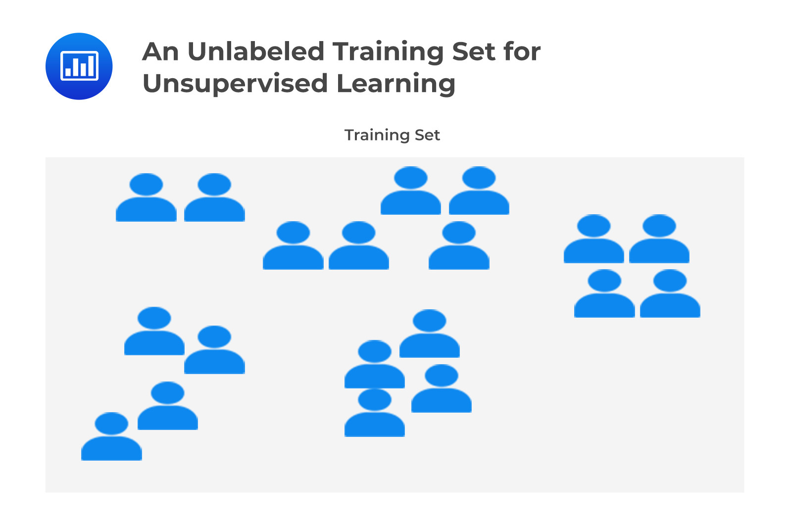
As the name suggests, the system attempts to learn without a teacher. It recognizes data patterns without an explicit target. More specifically, it uses inputs (X’s) for analysis with no corresponding target (Y). Data is clustered to detect groups or factors that explain the data. It is, therefore, not used for predictions.

For example, unsupervised learning can be used by an entrepreneur who sells books to detect groups of similar customers. The entrepreneur will at no point tell the algorithm which group a customer belongs to. It instead finds the connections without the entrepreneur’s help. The algorithm may notice, for instance, that 30% of the store’s customers are males who love science fiction books and frequent the store mostly during weekends, while 25% are females who enjoy drama books. A hierarchical clustering algorithm can be used to further subdivide groups into smaller ones.

Supervised Learning

Using well-labeled training data, this system is trained to work as a supervisor to teach the machine to predict the correct output. It works the same way a student learns under the supervision of a teacher. In supervised learning, a mapping function that can map inputs (X’s) with output (Y) is determined. The output is also known as the target, while X’s are also known as the features.

Typically, there are two types of tasks in supervised learning. One is classification. For example, a loan borrower may be classified as “likely to repay” or “likely to default.” The second one is the prediction of a target numerical value. For example, predicting a vehicle’s price based on a set of features such as mileage, year of manufacture, etc. For the latter, labels will indicate the selling prices. As for the former, the features would be the borrower’s credit score, income, etc., while the labels would be whether they defaulted.

Reinforcement Learning

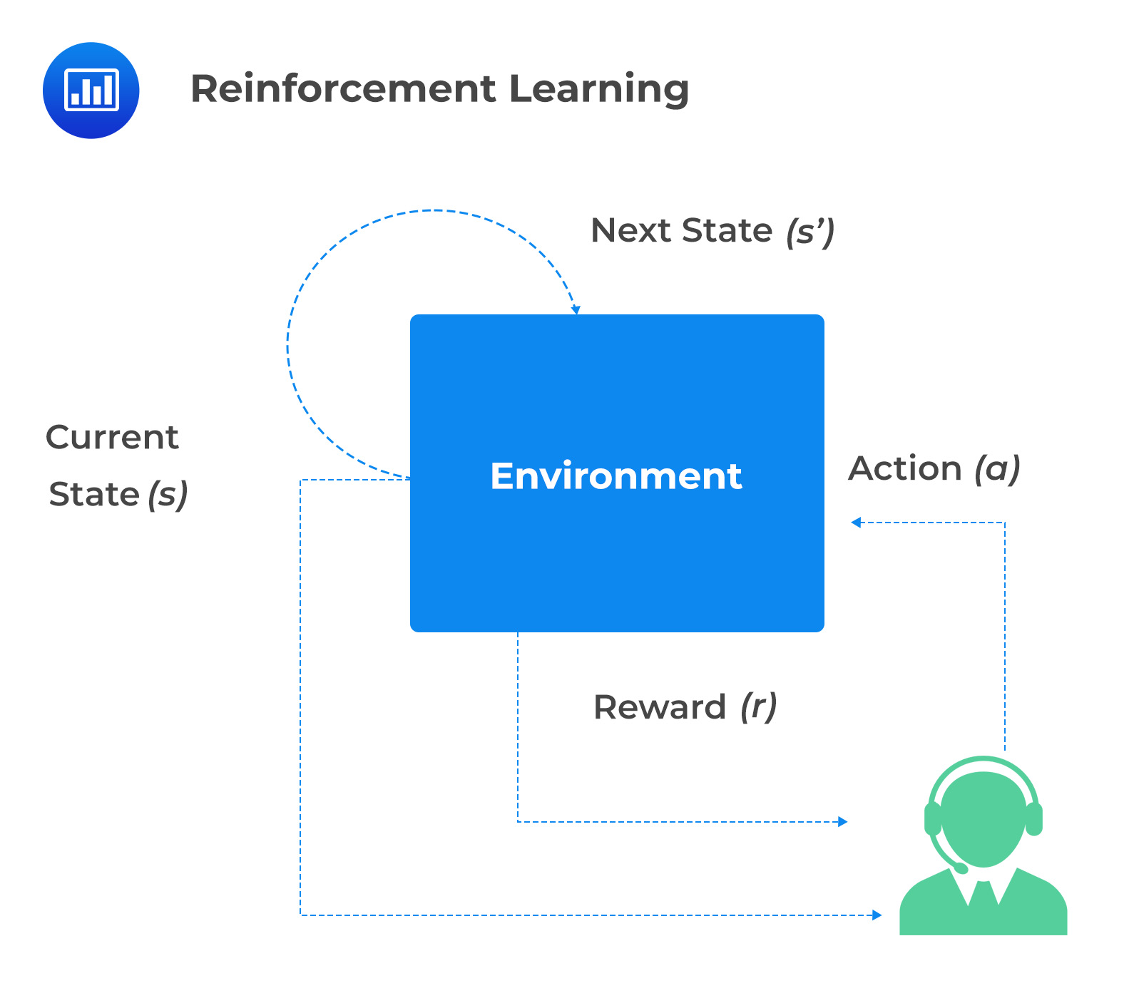
Reinforcement learning differs from other forms of learning. A learning system called an agent perceives and interprets its environment, performs actions, and is rewarded for desired behavior and penalized for undesired behavior. This is done through a trial-and-error approach. Over time, the agent learns by itself what is the best strategy (policy) that will generate the best reward while avoiding undesirable behaviors. Reinforcement learning can be used to optimize portfolio allocation and create trading bots that can learn from stock market data through trial and error, among many other uses.

In the next section, we will discuss how reinforcement learning operates and how it is used in decision-making.

How Reinforcement Learning Operates and How It’s Used in Decision-making

Reinforcement learning involves training an agent to make a series of decisions in an environment to maximize a reward. The agent is given feedback as either a reward or punishment depending on its actions. It then uses the feedback to learn the actions that are likely to generate the highest reward. The algorithm learns through trial and error by playing many times against itself.

How Reinforcement Learning Operates

Define the Environment

The environment consists of the state space, action space, and reward function. The state space is the set of all possible states in which the agent can be. On the other hand, the action space consists of a set of actions that the agent can take. Lastly, the reward function defines the feedback that the agent receives for taking a particular action in a given state space.

Initialize the Agent

Involves specifying the learning algorithm and any relevant parameters. The agent is then put in the original state of the environment.

Take an Action

The agent chooses an action depending on its current state and the learning algorithm. This action is then taken in the environment, which may lead to a change of state and a reward. At any given state, the algorithm can choose between taking the best course of action (exploitation) and trying a new action (exploration). Exploitation is assigned the probability \(p\), and exploration is given the probability \(1-p\). \(p\) increases as more trials are concluded, and the algorithm has learned more about the best strategy.

Update the Agent

Based on the agent’s reward and the environment’s new state, it updates its internal state. This update is carried out using some form of optimization algorithm.

Repeat the Process

The agent continues to take actions and update its internal state until it reaches a predefined number of iterations or a terminal state is reached.

Monte Carlo vs. Temporal Difference Methods for Reinforcement Learning

The Monte Carlo method estimates the value of a state or action based on the final reward received at the end of an episode. On the other hand, the temporal difference method updates the value of a state or action by looking at only one decision ahead when updating strategies.

An estimate of the expected value of taking action \(A\) in state \(S\), after several trials, is denoted as \(Q (S, A)\). The estimated value of being in state S at any time is expressed as:

$$\mathrm{Q}^{\text {new }}(\mathrm{S}, \mathrm{A})=\mathrm{Q}^{\text {old }}(\mathrm{S}, \mathrm{A})+\alpha\left[\mathrm{R}-\mathrm{Q}^{\text {old }}(\mathrm{S}, \mathrm{A})\right] $$

Where \(\alpha\) is a parameter, say \(0.05\), which is the learning rate that determines how much the agent updates its \(Q\) value based on the difference between the expected and actual reward.

Example: Reinforcement Learning

Suppose that we have three states \((S1 ,S2, S3)\) and two actions \((A1, A2)\), with the following \(Q(S,A)\) values:
\begin{array}{l|l|l|l}
 & S1 & S2 & S3 \\
\hline A1 & 0.3& 0.4& 0.5 \\
\hline A2 & 0.7 & 0.6 & 0.5 \\
 \end{array}

Monte-Carlo Method

Suppose that on the next trial, Action 2 is taken in State 3, and the total subsequent reward is 1.0. If \(\alpha= 0.075\), the Monte Carlo method would lead to \(Q (3,2)\) being updated from 0.5 to:

$$ \begin{align} Q(S3, A2) & =  Q(S3, A2) + 0.075 \times(1.0 – Q(S3, A2)) \\ &  =0.5 + 0.075(1.0 − 0.5) = 0.5375 \end{align} $$

Temporal Difference Method

If the next decision that has to be made on the trial under consideration happens when we are in State 2. Additionally, a reward of 0.3 is earned between the two decisions.

The value of being in State 2, Action 2 is 0.6. The temporal difference method would lead to \(Q (3,2)\) being updated from 0.5 to:

$$ 0.5+ 0.075(0.3 + 0.6 – 0.5) = 0.53 $$

Potential Applications of Reinforcement Learning in Finance

1. Trading: Reinforcement learning algorithms can learn from past data and market dynamics to make informed decisions on when to buy and sell, possibly optimizing the trading of financial instruments, including stocks, bonds, and derivatives.
2. Detecting fraud: RL can be used to detect fraudulent activity in financial transactions. This algorithm learns from past data and hence adapts to new fraud patterns. This means that the algorithm becomes better at detecting and preventing fraud with time.
3. Credit scoring: RL can be used to predict the probability of a borrower defaulting on a loan. The algorithm can be trained on historical data about borrowers and their credit histories to achieve this.
4. Risk management: RL can be trained using past data to identify and mitigate financial risks.
5. Portfolio optimization: RL can be trained to take actions that modify the allocation of assets in the portfolio with time, with the sim of maximizing portfolio returns and minimizing risks.

Practice Question

Which of the following is least likely a task that can be performed using natural language processing?

1. Sentiment analysis.
2. Text translation.
3. Image recognition.
4. Text classification.

Solution

The correct answer is C.

Image recognition is not a task that can be performed using NLP. This is because NLP is focused on understanding and processing text, not images.

A is incorrect: NLP can be used for sentiment analysis. For example, NLP can be used to measure the public opinion of a company, industry, or market trend by analyzing sentiments on social media posts.

B is incorrect: Financial documents may need to be translated into different languages to reach a global audience.

D is incorrect: Text classification is the process of assigning text data to prespecified categories. For example, text classification could involve assigning newswire statements based on the news they represent, e.g., education, financial, environmental, etc.