Characterizing Cycles

After completing this reading you should be able to:

• Define covariance stationary, autocovariance function, autocorrelation function, partial autocorrelation function, and autoregression.
• Describe the requirements for a series to be covariance stationary.
• Explain the implications of working with models that are not covariance stationary.
• Define white noise, and describe independent white noise and normal (Gaussian) white noise.
• Explain the characteristics of the dynamic structure of white noise.
• Explain how a lag operator works.
• Describe Wold’s theorem.
• Define a general linear process.
• Relate rational distributed lags to Wold’s theorem.
• Calculate the sample mean and sample autocorrelation, and describe the Box-Pierce Q-statistic and the Ljung-Box Q-statistic.
• Describe sample partial autocorrelation.

Covariance Stationery Time Series

The ordered set: \(\left\{ \dots ,{ y }_{ -2 },{ y }_{ -1 },{ y }_{ 0 },{ y }_{ 1 },{ y }_{ 2 },\dots \right\} \) is called the realization of a time series. Theoretically, it starts from the infinite past and proceeds to the infinite future. However, only a finite subset of realization can be used in practically, and is called a sample path.

A series is said to be covariance stationery if both its mean and covariance structure are stable over time. This implies that:

At time \(t\) the mean is:

$$ E\left( { y }_{ t } \right) ={ \mu }_{ t } $$

As covariance stationarity dictates, a mean that is stable over time is written as:

$$ E\left( { y }_{ t } \right) ={ \mu },\quad \quad \quad \forall t $$

It can be quite challenging to quantify the stability of a covariance structure. We will, therefore, use the autocovariance function. The covariance between \({ y }_{ t }\) and \({ y }_{ t-\tau }\) is the autocovariance at displacement \(\tau\). That is:

$$ \gamma \left( t,\tau \right) =cov\left( { y }_{ t },{ y }_{ t-\tau } \right) =E\left( { y }_{ t }-\mu \right) \left( { y }_{ t-\tau }-\mu \right) $$

As covariance stationarity demands, for autocovariance to solely depend on displacement, \(\tau\), then there must be stability in the covariance structure.

Therefore:

$$ \gamma \left( t,\tau \right) =\gamma \left( \tau \right) ,\quad \quad \quad \forall t $$

In a covariance stationery series, the cyclical functions are basically summarized by the autocovariance function. Autocovariances are graphed and examined as functions of \(\tau\). The function is symmetrical:

$$ \gamma \left( \tau \right) =\gamma \left( -\tau \right) ,\quad \quad \quad \forall t $$

Since displacement is the only factor that affects the autocovariance of a covariance stationery series, then the aspect of symmetry comes in.

Note that:

$$ \gamma \left( 0 \right) =cov\left( { y }_{ t },{ y }_{ t } \right) =var\left( { y }_{ t } \right) $$

This is another necessity of covariance stationarity. We must have a finite variance for the series. Furthermore, under covariance stationarity, other than being stable means should also be finite.

The correlation between two variables \(x\) and \(y\) can be defined as:

$$ corr\left( x,y \right) =\frac { cov\left( x,y \right) }{ { \sigma }_{ x }{ \sigma }_{ y } } $$

This implies that the product of the standard deviations of \(x\) and \(y\) normalizes or standardizes their covariance. The units of measurement of \(x\) and \(y\) do not affect the correlation. As compared to covariance, the correlation has a superior interpretability and is, therefore, more popular. The autocorrelation function, \(\rho \left( t \right) \), is applied more often than the autocovariance function, \(\gamma \left( \tau \right) \).

Where:

$$ \rho \left( t \right) =\frac { \gamma \left( \tau \right) }{ \gamma \left( 0 \right) } $$

And \(\tau =0,1,2,\dots \)

Note that \(\gamma \left( 0 \right)\) is the variance of \({ y }_{ t }\). Therefore, by covariance stationarity \(\gamma \left( 0 \right)\) is that variance of \(y\) at any other time \({ y }_{ t-1 }\).

Therefore:

$$ \rho \left( t \right) =\frac { cov\left( { y }_{ t },{ y }_{ t-1 } \right) }{ \sqrt { var\left( { y }_{ t } \right) } \sqrt { var\left( { y }_{ t-1 } \right) } } $$

$$ =\frac { \gamma \left( \tau \right) }{ \sqrt { \gamma \left( 0 \right) } \sqrt { \gamma \left( 0 \right) } } =\frac { \gamma \left( \tau \right) }{ \gamma \left( 0 \right) } $$

Note that:

$$ \rho \left( 0 \right) =\frac { { \gamma \left( 0 \right) } }{ { \gamma \left( 0 \right) } } =1 $$

The partial autocorrelation function is denoted as, \(p\left( \tau \right) \), and in a population linear regression of \({ y }_{ t }\) on \({ y }_{ t-1 },\dots ,{ y }_{ t-\tau }\), it is the coefficient of \({ y }_{ t-\tau }\). This regression is referred to as the autoregression. This is because the regression is on the lagged values of the variable.

White Noise

Assume that:

$$ { y }_{ t }={ \epsilon }_{ t } $$

$$ { \epsilon }_{ t }\sim \left( 0,{ \sigma }^{ 2 } \right) ,\quad \quad \quad \forall { \sigma }^{ 2 }<\infty $$

where \({ \epsilon }_{ t }\) is the shock and is uncorrelated over time. Therefore, \({ \epsilon }_{ t }\) and \({ y }_{ t }\) are said to be serially uncorrelated.

This that has a zero mean and unchanging variance is referred to as the zero-mean white noise (or just white noise) and is written as:

$$ { \epsilon }_{ t }\sim WN\left( 0,{ \sigma }^{ 2 } \right) $$

And:

$$ { y }_{ t }\sim WN\left( 0,{ \sigma }^{ 2 } \right) $$

\({ \epsilon }_{ t }\) and \({ y }_{ t }\) serially uncorrelated but not necessarily serially independent. If \(y\) possesses this property, (serially uncorrelated but not necessarily serially independent) then it is said to be an independent white noise.

Therefore, we write:

$$ { y }_{ t }\underset { \sim }{ iid } \left( 0,{ \sigma }^{ 2 } \right) $$

This is read as “\(y\) is independently and identically distributed with a mean and constant variance. \(y\) is said to be serially independent if it is serially uncorrelated and it has a normal distribution. In this case, \(y\) is called the normal white noise or the Gaussian white noise.

Written as:

$$ { y }_{ t }\underset { \sim }{ iid } N\left( 0,{ \sigma }^{ 2 } \right) $$

To characterize the dynamic stochastic structure of \({ y }_{ t }\sim WN\left( 0,{ \sigma }^{ 2 } \right) \), it follows that the unconditional mean and variance of \(y\) are:

$$ E\left( { y }_{ t } \right) =0 $$

And:

$$ var\left( { y }_{ t } \right) ={ \sigma }^{ 2 } $$

These two are constant since only displacement affects the autocovariances rather than time. All the autocovariances and autocorrelations are zero beyond displacement zero since white noise is uncorrelated over time.

The following is the autocovariance function for a white noise process:

$$ \gamma \left( \tau \right) =\begin{cases} { \sigma }^{ 2 },\quad \tau =0 \\ 0,\quad \quad \tau \ge 0\quad \quad \end{cases} $$

The following is the autocorrelation function for a white noise process:

$$ \rho \left( \tau \right) =\begin{cases} 1,\quad \quad \tau =0 \\ 0,\quad \quad \tau \ge 1\quad \end{cases} $$

Beyond displacement zero, all partial autocorrelations for a white noise process are zero. Thus, by construction white noise is serially uncorrelated. The following is the function of the partial autocorrelation for a white noise process:

$$ p\left( \tau \right) =\begin{cases} 1,\quad \quad \tau =0 \\ 0,\quad \quad \tau \ge 1\quad \end{cases} $$

Simple transformations of white noise are considered in the construction of processes with much richer dynamics. Then the white noise should be the 1-step-ahead forecast errors from good models.

The mean and variance of a process, conditional on its past is another crucial characterization of dynamics with crucial implications for forecasting.

To compare the conditional and unconditional means and variances, consider the independence white noise: \({ y }_{ t }\underset { \sim }{ iid } \left( 0,{ \sigma }^{ 2 } \right) \). \(y\) has an unconditional mean and variance of zero and \({ \sigma }^{ 2 }\) respectively. Now, consider the transformational set:

$$ { \Omega }_{ t-1 }=\left\{ { y }_{ t-1 },{ y }_{ t-2 },\dots \right\} $$

Or:

$$ { \Omega }_{ t-1 }=\left\{ { \epsilon }_{ t-1 },{ \epsilon }_{ t-2 },\dots \right\} $$

The conditional mean and variance do not necessarily have to be constant. The conditional mean for the independent white noise process is:

$$ E\left( { y }_{ t }|{ \Omega }_{ t-1 } \right) =0 $$

The conditional variance is:

$$ var\left( { y }_{ t }|{ \Omega }_{ t-1 } \right) =E\left( { \left( { y }_{ t }-E\left( { y }_{ t }|{ \Omega }_{ t-1 } \right) \right) }^{ 2 }|{ \Omega }_{ t-1 } \right) ={ \sigma }^{ 2 } $$

Independent white noise series have identical conditional and unconditional means and variances.

The Lag Operator

Let \(L\) denote the lag operator. This operator lags a series, as suggested by its name.

$$ L{ y }_{ t }={ y }_{ t-1 } $$

Furthermore:

$$ { L }^{ 2 }{ y }_{ t }=L\left( { L }{ y }_{ t } \right) =L\left( { y }_{ t-1 } \right) ={ y }_{ t-2 } $$

We apply the polynomial in the lag operator to operate on the series rather than the lag operator itself. A degree \(m\) polynomial in the lag operator is a linear function of powers of \(L\) to the \(m\)th factor.

That is:

$$ B\left( L \right) ={ b }_{ 0 }+{ b }_{ 1 }L+{ b }_{ 2 }{ L }^{ 2 }+\cdots +{ b }_{ m }{ L }^{ m } $$

Consider the following \(m\)th-order lag operator polynomial \({ L }^{ m }\), where:

$$ { { L }^{ m } }{ y }_{ t }={ y }_{ t-m } $$

This is a simple example of the operation on a series by a lag operator polynomial.

Let \(\Delta\) be the first-difference operator, then:

$$ \Delta { y }_{ t }=\left( 1-L \right) { y }_{ t }={ y }_{ t }-{ y }_{ t-1 } $$

The infinite-order lag polynomial operator is written as:

$$ B\left( L \right) ={ b }_{ 0 }+{ b }_{ 1 }L+{ b }_{ 2 }{ L }^{ 2 }+\cdots =\sum _{ i=0 }^{ \infty }{ { b }_{ i }{ L }^{ i } } $$

The following equation denotes the infinite distributed lag of current and past shocks:

$$ B\left( L \right) { \epsilon }_{ t }={ b }_{ 0 }{ \epsilon }_{ t }+{ b }_{ 1 }{ \epsilon }_{ t-1 }+{ b }_{ 2 }{ \epsilon }_{ t-2 }+\cdots =\sum _{ i=0 }^{ \infty }{ { b }_{ i }{ \epsilon }_{ t-i } } $$

Wold’s Theorem, the General Linear Process, and Rational Distributed Lags

Wold’s representation theorem will help us determine the appropriate model for a covariance stationary residual.

Wold’s Theorem

Assuming that \(\left\{ { y }_{ t } \right\} \) is any zero-mean covariance-stationary process. Then:

$$ { y }_{ t }=B\left( L \right) { \epsilon }_{ t }=\sum _{ i=0 }^{ \infty }{ { b }_{ i }{ \epsilon }_{ t-i } } $$

Where:

$$ { \epsilon }_{ t }\sim WN\left( 0,{ \sigma }^{ 2 } \right) $$

Note that \({ b }_{ 0 }=1\) and \({ \Sigma }_{ i=0 }^{ \infty }{ b }_{ i }^{ 2 }<0\).

The accurate model for any covariance stationery series is the Wold’s representation. Since \({ \epsilon }_{ t }\) corresponds to the 1-step-ahead forecast errors to be incurred should a particularly good forecast be applied, the \({ \epsilon }_{ t }\)’s are the innovations.

The General Linear Process

According to Wold’s theorem, the following is the only form of models to be considered when forecasting models for covariance stationary time series are formulated:

$$ { y }_{ t }=B\left( L \right) { \epsilon }_{ t }=\sum _{ i=0 }^{ \infty }{ { b }_{ i }{ \epsilon }_{ t-i } } $$

$$ { \epsilon }_{ t }\sim WN\left( 0,{ \sigma }^{ 2 } \right) $$

Where \({ b }_{ i }\) are the coefficients with \({ b }_{ 0 }=1\) and \({ \Sigma }_{ i=0 }^{ \infty }{ b }_{ i }^{ 2 }<0\). This is referred to as the general linear process.

Taking means and variances, the following unconditional moments are obtained:

$$ E\left( { y }_{ t } \right) =E\left( \sum _{ i=0 }^{ \infty }{ { b }_{ i }{ \epsilon }_{ t-i } } \right) =\sum _{ i=0 }^{ \infty }{ { b }_{ i }E\left( { \epsilon }_{ t-i } \right) } =\sum _{ i=0 }^{ \infty }{ { b }_{ i }\times 0 } =0 $$

And:

$$ var\left( { y }_{ t } \right) =var\left( \sum _{ i=0 }^{ \infty }{ { b }_{ i }{ \epsilon }_{ t-i } } \right) =\sum _{ i=0 }^{ \infty }{ { b }_{ i }^{ 2 }var\left( { \epsilon }_{ t-i } \right) } =\sum _{ i=0 }^{ \infty }{ { b }_{ i }^{ 2 }{ \sigma }^{ 2 } } ={ \sigma }^{ 2 }\sum _{ i=0 }^{ \infty }{ { b }_{ i }^{ 2 } } $$

Consider the information set:

$$ { \Omega }_{ t-1 }=\left\{ { \epsilon }_{ t-1 },{ \epsilon }_{ t-2 },\dots \right\} $$

The conditional mean is:

$$ E\left( { y }_{ t }|{ \Omega }_{ t-1 } \right) =E\left( { \epsilon }_{ t }|{ \Omega }_{ t-1 } \right) +{ b }_{ 1 }E\left( { \epsilon }_{ t }|{ \Omega }_{ t-1 } \right) +{ b }_{ 2 }E\left( { \epsilon }_{ t-2 }|{ \Omega }_{ t-1 } \right) +\cdots $$

$$ =0+{ b }_{ 1 }{ \epsilon }_{ t-1 }+{ b }_{ 2 }{ \epsilon }_{ t-2 }+\cdots =\sum _{ i=0 }^{ \infty }{ { b }_{ i }{ \epsilon }_{ t-i } } $$

The conditional variance is:

$$ var\left( { y }_{ t }|{ \Omega }_{ t-1 } \right) =E\left( { \left( { y }_{ t }-E\left( { y }_{ t }|{ \Omega }_{ t-1 } \right) \right) }^{ 2 }|{ \Omega }_{ t-1 } \right) =E\left( { \epsilon }_{ t }^{ 2 }|{ \Omega }_{ t-1 } \right) =E\left( { \epsilon }_{ t }^{ 2 } \right) ={ \sigma }^{ 2 } $$

Rational Distributed Lags

It is not a necessity that in the lag operator infinitely many free parameters be contained, by infinite polynomials, as they hinder its practical application. Such polynomials are often referred to as the rational polynomials. The rational distributed lags are the distributed lags built from them.

Let:

$$ B\left( L \right) =\frac { \Theta L }{ \Phi L } $$

The degree of the numerator polynomial is \(q\):

$$ \Theta L=\sum _{ i=0 }^{ q }{ { \theta }_{ i }{ L }^{ i } } $$

And the degree of the denominator polynomial is \(p\):

$$ \Phi L=\sum _{ i=0 }^{ p }{ { \varphi }_{ i }{ L }^{ i } } $$

In the \(B\left( L \right)\) polynomial, there lack infinitely many parameters. In fact there are \(p + q\) parameters.

Let \(B\left( L \right)\) be approximately rational, that is:

$$ B\left( L \right) \approx \frac { \Theta L }{ \Phi L } $$

Then, an approximation of the Wold’s representation can be determined if the rational distributed lag is applied.

Estimation and Inference for the Mean, Autocorrelation, and Partial Autocorrelation Functions

Sample Mean:

A stationery covariance series has a mean given as:

$$ \mu =E{ y }_{ t } $$

According to the analog principle, estimators are developed by using sample averages in the place of expectations. Therefore, the sample mean estimates our population mean for a sample of size \(T\).

$$ \bar { y } =\frac { 1 }{ T } \sum _{ t=1 }^{ T }{ { y }_{ t } } $$

This estimate is necessary when estimating the autocorrelation function.

Sample Autocorrelations

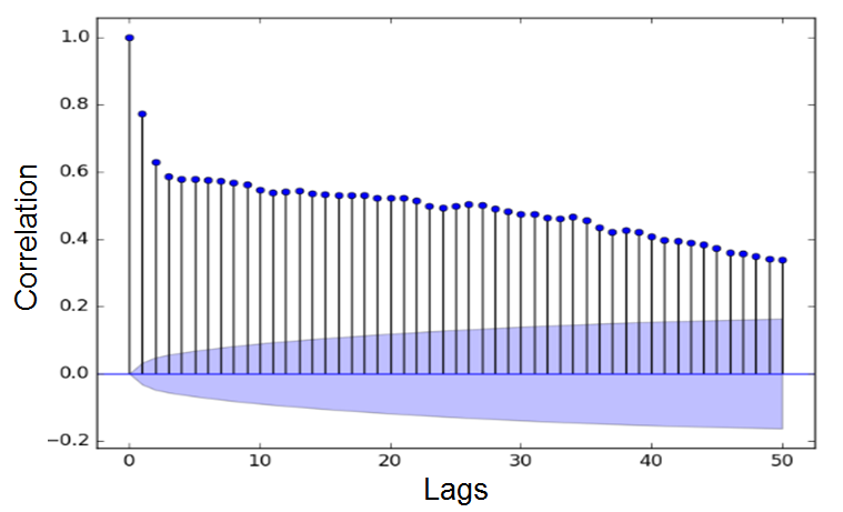
Consider the covariance stationary series \(y\), at the displacement \(\tau\) the autocorrelation is:

$$ \rho \left( \tau \right) =\frac { E\left( \left( { y }_{ t }-\mu \right) \left( { y }_{ t-\tau }-\mu \right) \right) }{ E\left( { \left( { y }_{ t }-\mu \right) }^{ 2 } \right) } $$

When the analog principle is applied, then the following is the natural estimator as a result:

$$ \hat { \rho } \left( \tau \right) =\frac { \frac { 1 }{ T } { \Sigma }_{ t=\tau +1 }^{ T }\left( \left( { y }_{ t }-\bar { y } \right) \left( { y }_{ t-\tau }-\bar { y } \right) \right) }{ \frac { 1 }{ T } { \Sigma }_{ t=1 }^{ T }{ \left( { y }_{ t }-\bar { y } \right) }^{ 2 } } =\frac { { \Sigma }_{ t=\tau +1 }^{ T }\left( \left( { y }_{ t }-\bar { y } \right) \left( { y }_{ t-\tau }-\bar { y } \right) \right) }{ { \Sigma }_{ t=1 }^{ T }{ \left( { y }_{ t }-\bar { y } \right) }^{ 2 } } $$

This estimator is referred to as the sample autocorrelation function or correlogram.

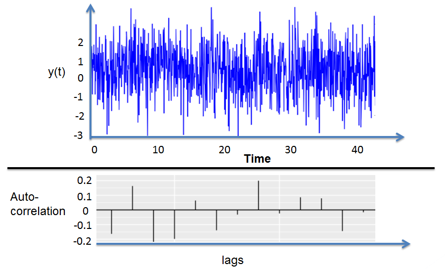
A series that is white noise has the following distribution of the sample autocorrelations in the large sample:

$$ \hat { \rho } \left( \tau \right) \sim N\left( 0,\frac { 1 }{ T } \right) $$

Since their mean is zero, the sample autocorrelations are the unbiased estimators of the true autocorrelations, which happen to be zero.

It is important to note that at various displacements, the sample autocorrelations are approximately independent of each other. The sum of independent \({ \chi }^{ 2 }\) variables is also \({ \chi }^{ 2 }\) degrees of freedom of the summed up variables.

The following is the equation for the Box-Pierce \(Q\)-Statistic:

$$ { Q }_{ BP }=T\sum _{ \tau =1 }^{ m }{ { \hat { \rho } }^{ 2 } } \left( \tau \right) $$

Under the null hypothesis that \(y\) is white noise, it is approximately it is approximately distributed as \({ \chi }_{ m }^{ 2 }\) random variable.

The following is a slight modification of the Box-Pierce \(Q\)-Statistic that closely follows the \({ \chi }^{ 2 }\) distribution in small samples:

$$ { Q }_{ LB }=T\left( T+2 \right) \sum _{ \tau =1 }^{ m }{ { \left( \widehat { \frac { 1 }{ T-\tau } } \right) } } { \rho }^{ 2 }\left( \tau \right) $$

The distribution of \({ Q }_{ LB }\) is approximately similar to that of \({ \chi }_{ m }^{ 2 }\) random variable if our null hypothesis is that \(y\) is white noise.

Apart from the fact that a weighted sum of squared autocorrelations replaces the sum of squared autocorrelations, then the Box-Pierce \(Q\)-Statistic is similar to the Ljung-Box \(Q\)-statistic. The weights here are:

$$ \frac { T+2 }{ T-\tau } $$

Sample Partial Autocorrelations

The sample partial autocorrelations correspond to a thought experiment involving linear regression using a sample of size \(T\).

Assume that the fitted regression is:

$$ { \hat { y } }_{ t }=\hat { c } +{ \hat { \beta } }_{ 1 }{ y }_{ t-1 }+\cdots +{ \hat { \beta } }_{ \tau }{ y }_{ t-\tau } $$

Therefore, at displacement \(\tau\), the following is the sample partial autocorrelation is:

$$ \hat { p } \left( \tau \right) ={ \hat { \beta } }_{ \tau } $$

Moving Averages (MA) Models

The moving average process of finite order is considered an approximation to the Wold representation that happens to be a moving average process of infinite order. Various sorts of shocks in a time series drive all variations.

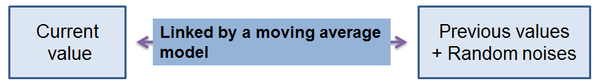The First-Order Moving Average (MA(1)) Process

The process is defined as:

$$ { y }_{ t }={ \epsilon }_{ t }+\theta { \epsilon }_{ t-1 }=\left( 1+\theta L \right) { \epsilon }_{ t } $$

$$ { \epsilon }_{ t }\sim WN\left( 0,{ \sigma }^{ 2 } \right) $$

In the general MA process, and particularly the MA(1) process, a function of current and lagged unobservable shocks expresses the current value of the observed series. This is an important feature that generally defines the MA process.

The following is the equation for the unconditional mean:

$$ E\left( { y }_{ t } \right) =E\left( { \epsilon }_{ t } \right) +\theta E\left( { \epsilon }_{ t-1 } \right) =0 $$

And the unconditional variance is:

$$ var\left( { y }_{ t } \right) =var\left( { \epsilon }_{ t } \right) +{ \theta }^{ 2 }var\left( { \epsilon }_{ t-1 } \right) ={ \sigma }^{ 2 }+{ \theta }^{ 2 }{ \sigma }^{ 2 }={ \sigma }^{ 2 }\left( 1+{ \theta }^{ 2 } \right) $$

An increase in the absolute value of \(\theta\) causes the unconditional variance to increase, given that the value of \(\sigma\) is constant.

Consider the following conditional information set:

$$ { \Omega }_{ t-1 }=\left\{ { \epsilon }_{ t-1 },{ \epsilon }_{ t-2 },\dots \right\} $$

The set has a conditional mean of:

$$ E\left( { y }_{ t }|{ \Omega }_{ t-1 } \right) =E\left( { \epsilon }_{ t }+\theta { \epsilon }_{ t-1 }|{ \Omega }_{ t-1 } \right) =E\left( { \epsilon }_{ t }|{ \Omega }_{ t-1 } \right) +\theta E\left( { \epsilon }_{ t }|{ \Omega }_{ t-1 } \right) =\theta { \epsilon }_{ t-1 } $$

And a conditional variance of:

$$ var\left( { y }_{ t }|{ \Omega }_{ t-1 } \right) =E\left( { \left( { y }_{ t }-E\left( { y }_{ t }|{ \Omega }_{ t-1 } \right) \right) }^{ 2 }|{ \Omega }_{ t-1 } \right) $$

$$ E\left( { \epsilon }_{ t }^{ 2 }|{ \Omega }_{ t-1 } \right) =E\left( { \epsilon }_{ t }^{ 2 } \right) ={ \sigma }^{ 2 } $$

The current conditional expectation is not affected whatsoever by more distant shocks, but only the first lag of the shock.

The next step is to calculate the autocorrelation of the MA(1) process. We start by calculating the autocovariance function. That is:

$$ \gamma \left( \tau \right) =E\left( { y }_{ t }{ y }_{ t-\tau } \right) =E\left( \left( { \epsilon }_{ t }+\theta { \epsilon }_{ t-1 } \right) \left( { \epsilon }_{ t-\tau }+\theta { \epsilon }_{ t-\tau -1 } \right) \right) $$

$$ =\begin{cases} \theta { \sigma }^{ 2 },\quad \quad \tau =1 \\ 0,\quad \quad \quad Otherwise \end{cases} $$

Therefore, the autocorrelation function is defined as:

$$ \rho \left( \tau \right) =\frac { \gamma \left( \tau \right) }{ \gamma \left( 0 \right) } =\begin{cases} \frac { \theta }{ 1+{ \theta }^{ 2 } } , & \tau =1 \\ 0, & Otherwise \end{cases} $$

This function happens to be the autocovariance function scaled by the variance.

The sharp cutoff in the autocorrelation function is a crucial feature in this case. Regardless of the values of MA parameters, the necessities for covariance stationarity for any MA(1) process are always met.

The MA(1) process is considered invertible if:

$$ |\theta |<1 $$

Therefore, the MA(1) process can be inverted and the current value of the series expressed in terms of a current shock and the lagged values of the series, instead of a current and a lagged shock. This is referred to as the autoregressive representation, and it can be calculated as follows:

The process has been defined as:

$$ { y }_{ t }={ \epsilon }_{ t }+\theta { \epsilon }_{ t-1 } $$

$$ { \epsilon }_{ t }\sim WN\left( 0,{ \sigma }^{ 2 } \right) $$

We then solve for the innovation:

$$ { \epsilon }_{ t }={ y }_{ t }-\theta { \epsilon }_{ t-1 } $$

The expressions for the innovations at various dates are given as follows after lagging by successively more periods:

$$ { \epsilon }_{ t-1 }={ y }_{ t-1 }-\theta { \epsilon }_{ t-2 } $$

$$ { \epsilon }_{ t-2 }={ y }_{ t-2 }-\theta { \epsilon }_{ t-3 } $$

$$ { \epsilon }_{ t-3 }={ y }_{ t-3 }-\theta { \epsilon }_{ t-4 } $$

After backward substitution in the MA(1) process we have:

$$ { y }_{ t }={ \epsilon }_{ t }+\theta { y }_{ t-1 }-{ \theta }^{ 2 }{ y }_{ t-2 }+{ \theta }^{ 3 }{ y }_{ t-3 }-\cdots $$

The finite autoregressive representation can be expressed as follows using the lag operator notation:

$$ \frac { 1 }{ 1+\theta L } { y }_{ t }={ \epsilon }_{ t } $$

Since \(\theta\), in the back substitution, is raised to some progressively higher powers, if \(|\theta |<1\) only then will a convergent autoregressive representation exist.

The only root of the MA(1) lag operator polynomial is the solution to:

$$ 1+{\theta L}=0 $$

Which is:

$$ L=-\frac { 1 }{ \theta } $$

This implies that if \(|\theta |<1\) then its inverse will be lower than 1 in absolute value.

The next step is to evaluate the partial autocorrelation function for the MA(1) process. This function will have a gradual decay to zero. In a sequence of progressive higher-order autoregressive approximations, the coefficients on the last included lag are the partial autocorrelations.

We have shown that for the general autoregressive representation:

$$ { y }_{ t }={ \epsilon }_{ t }+\theta { y }_{ t-1 }-{ \theta }^{ 2 }{ y }_{ t-2 }+{ \theta }^{ 3 }{ y }_{ t-3 }-\cdots $$

When \(\theta=0.5\) we have that:

$$ { y }_{ t }={ \epsilon }_{ t }+0.5{ y }_{ t-1 }-{ 0.5 }^{ 2 }{ y }_{ t-2 }+{ 0.5 }^{ 3 }{ y }_{ t-3 }-\cdots $$

A similar damped oscillation is observed for the partial autocorrelations.

The Finite-Order Moving Average Process of order \(q\), MA(\(q\)), Process

For MA(\(q\)) process, we have that:

$$ { y }_{ t }={ \epsilon }_{ t }+{ \theta }_{ 1 }{ \epsilon }_{ t-1 }+\cdots +{ \theta }_{ q }{ \epsilon }_{ t-q }=\Theta \left( L \right) { \epsilon }_{ t } $$

$$ { \epsilon }_{ t }\sim WN\left( 0,{ \sigma }^{ 2 } \right) $$

The \(q\)th-order lag operator polynomial is given as, \(\Theta \left( L \right)\).

Where:

$$ \Theta \left( L \right) =1+{ \theta }_{ 1 }L+\cdots +{ \theta }_{ q }{ L }^{ q } $$

The MA(\(q\)) process is a generalized representation of the MA(1) process. This means that the MA(1) process is a special case of the MA(\(q\)) process, with \(q\) being equal to 1.

Therefore, the MA(\(q\)) and the MA(1) processes have properties that are similar in all aspects. When \(q>1\), the MA(\(q\)) lag operator polynomial has \(q\) roots, and there are chances of ending up with complex roots.

For invertibility of the MA(\(q\)) process to exist, all the roots must have inverses that are inside the unit circle. This enables us to have the convergent autoregressive representation:

$$ \frac { 1 }{ \Theta \left( L \right) } { y }_{ t }={ \epsilon }_{ t } $$

Depending on the information set, the MA(\(q\)) process’ conditional mean changes accordingly. However, the unconditional moments are fixed. The \(q\) lags of the innovation in the MA(\(q\)) process are the determining factors for the conditional mean. This makes the MA(\(q\)) process have a potentially longer memory, which is clearly observed in its autocorrelation function where all the autocorrelations are zero, beyond the \(q\)th displacement.

The defining property of the moving average process is this autocorrelation cutoff.

According to Wold’s representation:

$$ { y }_{ t }=B\left( L \right) { \epsilon }_{ t } $$

With the order of \(B\left( L \right)\) being infinite. The infinite order polynomial \(B\left( L \right)\) is approximated by applying the first order polynomial \(1+{ \theta }L\), as the MA(1) model is being fit.

Even better approximations to the Wold representation can be provided by the MA(\(q\)) processes. The infinite moving average is approximated by the MA(\(q\)) process, with a moving average of finite order,

$$ { y }_{ t }=\Theta \left( L \right) { \epsilon }_{ t }. $$

Autoregressive Models (AR) Models

This another approximation to the Wold representation. The autoregressive process is a simple stochastic difference equation. In discrete time-stochastic dynamic modeling, the natural vehicle is the stochastic difference equations.

The AR(1) process

The following equation is the AR(1) for short, in the AR(1) process:

$$ { y }_{ t }={ \epsilon }_{ t }+\varphi { y }_{ t-1 } $$

$$ { \epsilon }_{ t }\sim WN\left( 0,{ \sigma }^{ 2 } \right) $$

It can also be expressed in the lag operator form as follows:

$$ \left( 1-\varphi L \right) { y }_{ t }={ \epsilon }_{ t } $$

It is also important to note that a finite-order moving average process is always covariant stationary. However, for invertibility, certain conditions have to be met. But for autoregressive process invertibility always exist. However, covariance stationarity in the autoregressive process requires some conditions to be satisfied.

For the AR(1) process:

$$ { y }_{ t }=\varphi { y }_{ t-1 }+{ \epsilon }_{ t } $$

Then on the right hand side backward substitution for the lagged \(y\)’s is done to obtain:

$$ { y }_{ t }={ \epsilon }_{ t }+\varphi { \epsilon }_{ t-1 }+{ \varphi }^{ 2 }{ \epsilon }_{ t-2 }+\cdots $$

And this can be expressed in the following manner in the lag operator form:

$$ { y }_{ t }=\frac { 1 }{ 1-\varphi L } { \epsilon }_{ t } $$

For convergence to exist in this moving average representation for \(y\), then \(|\varphi |<1\). Therefore, in the AR(1) process, the condition for covariance stationarity is \(|\varphi |<1\).

The unconditional mean can be calculated as:

$$ E\left( { y }_{ t } \right) =E\left( { \epsilon }_{ t }+\varphi { \epsilon }_{ t-1 }+{ \varphi }^{ 2 }{ \epsilon }_{ t-2 }+\cdots \right) $$

$$ =E\left( { \epsilon }_{ t } \right) +\varphi E\left( { \epsilon }_{ t-1 } \right) +{ \varphi }^{ 2 }E\left( { \epsilon }_{ t-2 } \right) +\cdots $$

$$ =0 $$

And the unconditional variance is calculated as:

$$ var\left( { y }_{ t } \right) =var\left( { \epsilon }_{ t }+\varphi { \epsilon }_{ t-1 }+{ \varphi }^{ 2 }{ \epsilon }_{ t-2 }+\cdots \right) $$

$$ ={ \sigma }^{ 2 }+{ \varphi }^{ 2 }{ \sigma }^{ 2 }+{ \varphi }^{ 4 }{ \sigma }^{ 2 }+\cdots $$

$$ ={ \sigma }^{ 2 }\sum _{ i=0 }^{ \infty }{ { \varphi }^{ 2i } } $$

$$ = \frac { { \sigma }^{ 2 } }{ 1-{ \varphi }^{ 2 } } $$

The conditional moments are:

$$ E\left( { y }_{ t }|{ y }_{ t-1 } \right) =E\left( \varphi { y }_{ t-1 }+{ \epsilon }_{ t }|{ y }_{ t-1 } \right) $$

$$ =\varphi E\left( { y }_{ t-1 }|{ y }_{ t-1 } \right) +E\left( { \epsilon }_{ t }|{ y }_{ t-1 } \right) $$

$$ =\varphi { y }_{ t-1 }+0 $$

$$ =\varphi { y }_{ t-1 } $$

And:

$$ Var\left( { y }_{ t }|{ y }_{ t-1 } \right) =var\left( \varphi { y }_{ t-1 }+{ \epsilon }_{ t }|{ y }_{ t-1 } \right) $$

$$ ={ \varphi }^{ 2 }var\left( { y }_{ t-1 }|{ y }_{ t-1 } \right) +var\left( { \epsilon }_{ t }|{ y }_{ t-1 } \right) $$

$$ =0+{ \sigma }^{ 2 } $$

$$ ={ \sigma }^{ 2 } $$

For the autocovariances we have:

$$ { y }_{ t }=\varphi { y }_{ t-1 }+{ \epsilon }_{ t } $$

Both sides of the equation are multiplied by \({ y }_{ t-\tau }\), such that:

$$ { y }_{ t }\times { y }_{ t-\tau }=\varphi \times { y }_{ t-\tau }\times { y }_{ t-1 }+{ y }_{ t-\tau } \times { \epsilon }_{ t } $$

For \(\tau \ge 1\),when we take expectations of both sides we obtain:

$$ \gamma \left( \tau \right) =\varphi \gamma \left( \tau -1 \right) $$

This results in the Yule-Walker Equation: Given \(\gamma \left( \tau \right)\), for any \(\tau\) , \(\gamma \left( \tau -1 \right)\) can be obtained in accordance with the Yule-Walker equation. Let \(\gamma \left( 0 \right)\) be the variance of the process, such that:

$$ \gamma \left( 0 \right) =\frac { { \sigma }^{ 2 } }{ 1-{ \varphi }^{ 2 } } $$

$$ \gamma \left( 1 \right) =\varphi \frac { { \sigma }^{ 2 } }{ 1-{ \varphi }^{ 2 } } $$

$$ \gamma \left( 2 \right) ={ \varphi }^{ 2 }\frac { { \sigma }^{ 2 } }{ 1-{ \varphi }^{ 2 } } $$

This can be generally expressed as:

$$ \gamma \left( \tau \right) ={ \varphi }^{ \tau }\frac { { \sigma }^{ 2 } }{ 1-{ \varphi }^{ 2 } } ,\quad \quad \quad \tau =0,1,2,\dots $$

We then divide through by \(\gamma \left( 0 \right)\) and we obtain the autocorrelations,

$$ \rho \left( \tau \right) ={ \varphi }^{ \tau },,\quad \quad \quad \quad \tau =0,1,2,\dots $$

A positive \(\varphi\) implies a one-sided autocorrelation decay, while a negative \(\varphi\) implies that the decay is about back and forth oscillations.

The AR(1) process has a partial autocorrelation function that cuts off abruptly.

Therefore:

$$ \rho \left( \tau \right) =\begin{cases} \varphi , & \tau =1 \\ 0, & \tau >1 \end{cases} $$

The first partial autocorrelation is the autoregressive coefficient, with all the longer lags having coefficients of zero, for the true process that is an AR(1).

AR(\(p\)) Process

The following is the equation of a general \(p\)th order autoregressive process, AR(\(p\)):

$$ { y }_{ t }={ \varphi }_{ 1 }{ y }_{ t-1 }+{ \varphi }_{ 2 }{ y }_{ t-2 }+\cdots +{ \varphi }_{ p }{ y }_{ t-p }+{ \epsilon }_{ t } $$

$$ { \epsilon }_{ t }\sim WN\left( 0,{ \sigma }^{ 2 } \right) $$

This can also be expressed in the following way, as a lag operator:

$$ \Phi \left( L \right) { y }_{ t }=\left( 1-{ \varphi }_{ 1 }L-{ \varphi }_{ 2 }{ L }^{ 2 }-\cdots -{ \varphi }_{ p }{ L }^{ p } \right) { y }_{ t }={ \epsilon }_{ t } $$

Covariance stationarity in the AR(\(p\)) process occurs iff all the roots of the autoregressive lag operator polynomial \(\Phi \left( L \right)\) have inverses that fall inside the unit circle. Here, the process can be written in the form of a convergent infinite moving average:

$$ { y }_{ t }=\frac { 1 }{ \Phi \left( L \right) } { \epsilon }_{ t } $$

At displacement \(p\), the cutoff for the AR(\(p\)) partial autocorrelation is sharp.

Autoregressive Moving Average (ARMA) Models

These are models combined with a view of obtaining a better approximation to the Wold representation. The result is the autoregressive moving average, ARMA (\(p,q\)), process. The ARMA(1,1) is the simplest ARMA process which is neither a pure autoregression or a pure moving average. That is:

$$ { y }_{ t }=\varphi { y }_{ t-1 }+{ \epsilon }_{ t }+\theta { \epsilon }_{ t-1 } $$

$$ { \epsilon }_{ t }\sim WN\left( 0,{ \sigma }^{ 2 } \right) $$

Or as a lag operator:

$$ \left( 1-\varphi L \right) { y }_{ t }=\left( 1+\theta L \right) { \epsilon }_{ t } $$

For stationarity and invertibility, the absolute value of \(\theta\) should be less than one. With covariance stationarity, then the moving average representation is:

$$ { y }_{ t }=\frac { \left( 1+\theta L \right) }{ \left( 1-\varphi L \right) } { \epsilon }_{ t } $$

This happens to be an infinite distributed lag of current and past innovations. The following is the infinite autoregressive representation with the invertibility condition satisfied:

$$ \frac { \left( 1-\varphi L \right) }{ \left( 1+\theta L \right) } { y }_{ t }={ \epsilon }_{ t } $$

The ARMA(1,1) is a special case of the ARMA(\(p,q\)) process, such that:

$$ { y }_{ t }={ { \varphi }_{ 1 }y }_{ t-1 }+{ { \varphi }_{ 2 }y }_{ t-2 }+\cdots +{ { \varphi }_{ p }y }_{ t-p }+{ \epsilon }_{ t }+{ { \theta }_{ 1 }\epsilon }_{ t-1 }+{ { \theta }_{ 2 }\epsilon }_{ t-2 }+\cdots +{ { \theta }_{ q }\epsilon }_{ t-q } $$

$$ { \epsilon }_{ t }\sim WN\left( 0,{ \sigma }^{ 2 } \right) $$

Or:

$$ \Phi \left( L \right) { y }_{ t }=\Theta \left( L \right) { \epsilon }_{ t } $$

Where:

$$ \Phi \left( L \right) =1-{ \varphi }_{ 1 }L-{ \varphi }_{ 2 }{ L }^{ 2 }-\cdots { \varphi }_{ p }{ L }^{ p } $$

And:

$$ \Theta \left( L \right) =1+{ \theta }_{ 1 }L+{ \theta }_{ 2 }{ L }^{ 2 }+\cdots +{ \theta }_{ q }{ L }^{ q } $$

The process is considered covariance stationery with a convergent infinite moving average representation, in the event that all the inverses of the roots of \(\Phi \left( L \right)\) fall inside the unit circle.

That is:

$$ { y }_{ t }=\frac { \Theta \left( L \right) }{ \Phi \left( L \right) } { \epsilon }_{ t } $$

The process is considered invertible with a convergent infinite autoregressive representation, in the event that all the inverses of the roots of \(\Theta \left( L \right)\) fall inside the unit circle.

That is:

$$ \frac { \Phi \left( L \right) }{ \Theta \left( L \right) } { y }_{ t }={ \epsilon }_{ t } $$

Application: Specifying and Estimating Models for Employment Forecasting

Moving averages are nonlinear in parameters. We need to understand how they are nonlinear and their estimation. The following is an invertible MA(1) model having a mean that is not zero:

$$ { y }_{ t }=\mu +{ \epsilon }_{ t }+\theta { \epsilon }_{ t-1 } $$

If we undertake an \(m\) times backward substitution, then the following autoregression approximation will be obtained:

$$ { y }_{ t }\approx \frac { \mu }{ 1+\theta } +\theta { y }_{ t-1 }-{ \theta }^{ 2 }{ y }_{ t-2 }+\cdots +{ \left( -1 \right) }^{ m-1 }{ \theta }^{ m }{ y }_{ t-m }+{ \epsilon }_{ t } $$

This implies that an invertible moving average can be approximated as an autoregression of finite-order, with better approximations being obtained when the value of \(m\) is increased. Therefore, the residuals can be expressed approximately in terms of the observed data and then solve for the parameters minimizing the sum of squared residuals, (using a computer):

$$ \hat { \mu } ,\hat { \theta } =\underset { \mu ,\theta }{ argmin } \sum _{ t=1 }^{ T }{ { \left( { y }_{ t }-\left( \frac { \mu }{ 1+\theta } +\theta { y }_{ t-1 }-{ \theta }^{ 2 }{ y }_{ t-2 }+\cdots +{ \left( -1 \right) }^{ m-1 }{ \theta }^{ m }{ y }_{ t-m } \right) \right) }^{ 2 } } $$

$$ { \hat { \sigma } }^{ 2 }=\frac { 1 }{ T } \sum _{ t=1 }^{ T }{ { \left( { y }_{ t }-\left( \frac { \hat { \mu } }{ 1+\hat { \theta } } +\hat { \theta } { y }_{ t-1 }-{ \hat { \theta } }^{ 2 }{ y }_{ t-2 }+\cdots +{ \left( -1 \right) }^{ m-1 }{ \hat { \theta } }^{ m }{ y }_{ t-m } \right) \right) }^{ 2 } } $$

We apply the numerical approximation models to determine the parameter estimates since the autoregressive approximation has restricted parameters.

There are also some alternative approximations of autoregressions is one of them. We can apply the ordinary least-squares regression to conveniently estimate the autoregressions.

Assuming that we have the following AR(1) model:

$$ \left( { y }_{ t }-\mu \right) =\varphi \left( { y }_{ t-1 }-\mu \right) +{ \epsilon }_{ t } $$

$$ { \epsilon }_{ t }\sim WN\left( 0,{ \sigma }^{ 2 } \right) $$

This can as well be written as:

$$ \left( { y }_{ t } \right) =c+\varphi { y }_{ t-1 }+{ \epsilon }_{ t } $$

And:

$$ c=\mu \left( 1-\varphi \right) $$

Then the least squares estimators will be:

$$ \hat { c } ,\hat { \mu } =\underset { c,\mu }{ argmin } \sum _{ t=1 }^{ T }{ { \left( { y }_{ t }-c-\varphi { y }_{ t-1 } \right) }^{ 2 } } $$

And:

$$ { \hat { \sigma } }^{ 2 }=\frac { 1 }{ T } \sum _{ t=1 }^{ T }{ { \left( { y }_{ t }-\hat { c } -\hat { \varphi } { y }_{ t-1 } \right) }^{ 2 } } $$

\(\mu\) has an implied estimate of:

$$ \hat { \mu } =\frac { \hat { c } }{ 1-\hat { \mu } } $$

Question 1

The following sample autocorrelation estimates are obtained using 300 data points: 

Compute the value of the Ljung-Box Q-statistic.

1. 22.5
2. 22.74
3. 30
4. 30.1

The correct answer is A.

$$ { Q }_{ BP }=T\sum _{ \tau =1 }^{ m }{ { \hat { \rho } }^{ 2 } } \left( \tau \right) $$

$$ = 300({0.25}^{ 2 }+ {(-0.1)}^{2}+ {(-0.05)}^{2}) = 22.5 $$

Question 2

The following sample autocorrelation estimates are obtained using 300 data points: 

Compute the value of the Box-Pierce Q-statistic.

1. 30.1
2. 30
3. 22.5
4. 22.74

The correct answer is D.

$$ { Q }_{ LB }=T\left( T+2 \right) \sum _{ \tau =1 }^{ m }{ { \left( \widehat { \frac { 1 }{ T-\tau } } \right) } } { \rho }^{ 2 }\left( \tau \right) $$

$$ = 300(302)({ \frac {{0.25}^{ 2 }}{299}} + { \frac {{-0.1}^{ 2 }}{298}} + { \frac {{-0.05}^{ 2 }}{297}} ) = 22.74 $$

Note: Provided the sample size is large, the Box-Pierce and the Ljung-Box tests typically arrive at the same result.

Question 3

Assume the shock in a time series is approximated by Gaussian white noise. Yesterday’s realization, y(t) was 0.015 and the lagged shock was -0.160. Today’s shock is 0.170.

If the weight parameter theta, θ, is equal to 0.70, determine today’s realization under a first-order moving average, MA(1), process.

1. -4.205
2. 4.545
3. 0.058
4. 0.282

The correct answer is C.

Today’s shock = \({ \epsilon }_{ t }\); yesterday’s shock = \({ \epsilon }_{ t-1 }\); today’s realization = \({ y }_{ t }\); yesterday’s realization = \({ y }_{ t-1 }\).

The MA(1) is given by:

$$ { y }_{ t }={ \epsilon }_{ t }+\theta { \epsilon }_{ t-1 } $$

$$ { y }_{ t }= 0.170 + 0.7(-0.160) = 0.058 $$