


Hypothesis Testing
After completing this reading, you should be able to: Construct an appropriate null... Read More
After completing this reading you should be able to:
Trend is a general systematic linear or (most often) nonlinear component that changes over time and does not repeat. It is a pattern of gradual change in a condition, output, or process, or an average or general tendency of a series of data points to move in a certain direction over time.
There are deterministic trend models whose evolution is perfectly predictable. These models are very important and are practically very applicable.
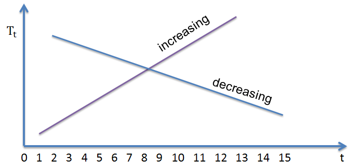
Consider the following linear time function:
$$ { T }_{ t }={ \beta }_{ 0 }+{ \beta }_{ 1 }{ TIME }_{ t } $$
This is a perfect example of a trend description equation. Note that the time trend or time dummy, denoted by the variable \(TIME\) is an artificial creation. A sample of size \(T\) has:
$$ { TIME }_{ t }=t $$
Where:
\( TIME=\left( 1,2,3,\dots ,T-1,T \right) \)
The regression intercept is denoted as \({ \beta }_{ 0 }\). At time \(t = 0\), the regression will equal to \({ \beta }_{ 0 }\). The regression slope is denoted as \({ \beta }_{ 1 }\). Note also that an increasing trend will have a positive slope while a decreasing one will have a negative slope. An increasing linear trend in the fields of business, finance, and economics usually indicate growth, but not always the case.
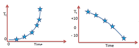
Trends may also take a nonlinear or curved form. A good example is a variable that increases at a rate that is increasing or declining. It is not a necessity that trends be linear, but rather they should be smooth.
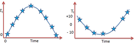
The other model is the quadratic trend model. These models are capable of catching nonlinearities. Consider the following function:
$$ { T }_{ t }={ \beta }_{ 0 }+{ \beta }_{ 1 }{ TIME }_{ t }+{ \beta }_{ 2 }{ Time }_{ t }^{ 2 } $$
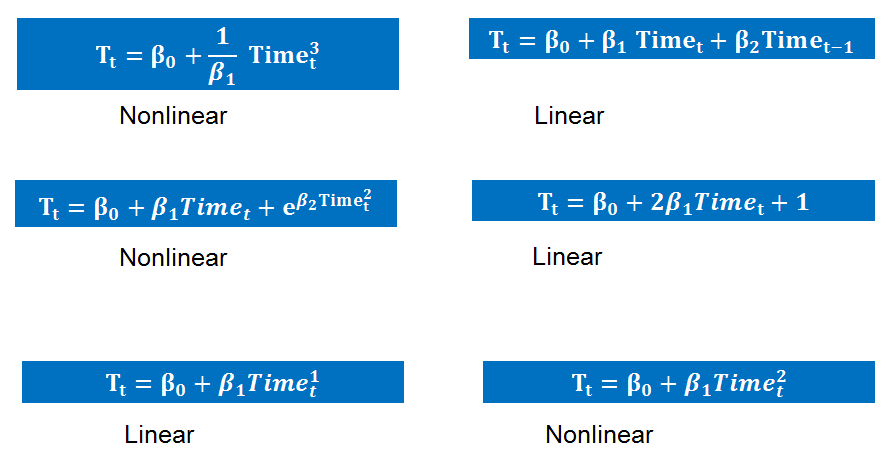
If \({ \beta }_{ 2 }=0\), then we have the emergence of a linear trend. If smoothness is to be maintained, then polynomials of lower order are applied. We may have several shapes of nonlinear trends. This will be determined by how large or small the coefficients are and whether they are positive or negative.
If both \({ \beta }_{ 1 }\) and \({ \beta }_{ 2 }\) have a positive sign then the trend increases in a monotonically and nonlinearly manner. On the other hand, if both \({ \beta }_{ 1 }\) and \({ \beta }_{ 2 }\) are less than zero then the trend decreases on a monotonically manner.
 The trend becomes U-shaped when \({ \beta }_{ 1 }\) is negative and \({ \beta }_{ 2 }\) is positive. We obtain an inverted U-shaped trend in the event that \({ \beta }_{ 1 }\) is positive and \({ \beta }_{ 2 }\) is negative.
The concept of exponential trend arises when the appearance of a trend is nonlinear in levels but linear in logarithms. It is also referred to as the log-linear trend. This is a very common occurrence in the fields of business, finance, and economics where growth is roughly constant, as indicated by the economic variables.
A trend with a constant growth rate at \({ \beta }_{ 1 }\) can be expressed as:
$$ { T }_{ t }={ \beta }_{ 0 }{ e }^{ { \beta }_{ 1 }{ Time }_{ t } } $$
In levels, this trend happens to an exponential, hence nonlinear, time function. However the same trend can be written as logarithms:
$$ ln\left( { T }_{ t } \right) =ln\left( { \beta }_{ 0 } \right) +{ \beta }_{ 1 }{ Time }_{ t } $$
Hence becoming a linear function of time.
The exponential trend is similar to the quadratic trend in the sense that we can have a variety of patterns depending on whether the parameter values are big or small whether they have a positive or negative sign. Their rate of increase or decrease can either decline or increase.
 There are subtle differences between qualitative trend shapes of similar sorts despite the fact that quadratic and exponential trends achieving them. Certain series can have quadratic trends approximating their nonlinear trends quite well. Yet for others, it is the exponential trend offer a better approximation.
It is important that variables such as time and its square be created and stored in a computer prior to estimating trend models.
Least squares regression is used to fit some trend models to data on a time series \(y\). We compute the following using a computer:
$$ \hat { \theta } =\underset { \theta }{ argmin } \sum _{ t=1 }^{ T }{ { \left( { y }_{ t }-{ T }_{ t }\left( \theta \right) \right) }^{ 2 } } $$
The set of parameters to be estimated are given as \( \theta\).
For a linear trend, we have that:
$$ { T }_{ t }\left( \theta \right) ={ \beta }_{ 0 }+{ \beta }_{ 1 }{ TIME }_{ t } $$
$$ \theta =\left( { \beta }_{ 0 },{ \beta }_{ 1 } \right) $$
Therefore, the computer determines:
$$ \left( { \hat { \beta } }_{ 0 },{ \hat { \beta } }_{ 1 } \right) =\underset { { \beta }_{ 0 },{ \beta }_{ 1 } }{ argmin } \sum _{ t=1 }^{ T }{ { \left( { y }_{ t }-{ \beta }_{ 0 }-{ \beta }_{ 1 }{ TIME }_{ t } \right) }^{ 2 } } $$
For a quadrative trend the computer determines:
$$ \left( { \hat { \beta } }_{ 0 },{ \hat { \beta } }_{ 1 },{ \hat { \beta } }_{ 2 } \right) =\underset { { \hat { \beta } }_{ 0 },{ \hat { \beta } }_{ 1 },{ \hat { \beta } }_{ 2 } }{ argmin } \sum _{ t=1 }^{ T }{ { \left( { y }_{ t }-{ \beta }_{ 0 }-{ \beta }_{ 1 }{ TIME }_{ t }-{ \beta }_{ 2 }{ TIME }_{ t }^{ 2 } \right) }^{ 2 } } $$
An exponential trend can be estimated in two ways. The first approach involves proceeding directly from the exponential representation and let the computer determine:
$$ \left( { \hat { \beta } }_{ 0 },{ \hat { \beta } }_{ 1 } \right) =\underset { { \beta }_{ 0 },{ \beta }_{ 1 } }{ argmin } \sum _{ t=1 }^{ T }{ { \left( { y }_{ t }-{ \beta }_{ 0 }{ e }^{ { \beta }_{ 1 }{ TIME }_{ t } } \right) }^{ 2 } } $$
In the second approach, log \(y\) is regressed on an intercept and \(TIME\). The computer therefore determines:
$$ \left( { \hat { \beta } }_{ 0 },{ \hat { \beta } }_{ 1 } \right) =\underset { { \beta }_{ 0 },{ \beta }_{ 1 } }{ argmin } \sum _{ t=1 }^{ T }{ { \left( { lny }_{ t }-ln{ \beta }_{ 0 }-{ \beta }_{ 1 }{ TIME }_{ t } \right) }^{ 2 } } $$
It is important to consider the fact that the fitted values from this are the fitted values of log \(y\). Therefore, the fitted values of \(y\) are obtained by their exponentiation.
Argmin just means “the argument that minimizes.” Least squares proceeds by finding the argument (in this case, the value of θ) that minimizes the sum of squared residuals; thus, the least squares estimator is the “argmin” of the sum of squared residuals function.
Point forecasts construction should be our first consideration. Assuming that currently, we are at time \(T\), and the \(h\)-step-ahead value of a series \(y\) should be forecasted by the use of a trend model. Consider the following linear model that holds for any time \(t\):
$$ { y }_{ t }={ \beta }_{ 0 }+{ \beta }_{ 1 }{ Time }_{ t }+{ \varepsilon }_{ t } $$
At time \(t + h\) we have:
$$ { y }_{ T+h }={ \beta }_{ 0 }+{ \beta }_{ 1 }{ Time }_{ T+h }+{ \varepsilon }_{ T+h } $$
On the right side of the equation we have two future value of series, \({ Time }_{ T+h }+{ \varepsilon }_{ T+h }\). Supposing that we knew \({ Time }_{ T+h }\) and \({ \varepsilon }_{ T+h }\) at time \(T\), then the forecast could be immediately cranked out. \({ Time }_{ T+h }\) being known could be attributed to the fact that the artificially constructed time variable is perfectly predictable.
However, since we do not know \({ \varepsilon }_{ T+h }\) at time \(T\), an optimal forecast of \({ \varepsilon }_{ T+h }\) is constructed using information up to time \(T\). \(\varepsilon\) assumed to be a simple independent zero-mean random noise. For any future period, the optimal forecast of \({ \varepsilon }_{ T+h }\) is zero. This results in the following point forecast:
$$ { y }_{ T+h,T }={ \beta }_{ 0 }+{ \beta }_{ 1 }{ Time }_{ T+h } $$
It is important to note that the subscript \({ T+h,T }\) informs us that the forecast is for time \(T+h\), and is made at time \(T\). This point forecast can be made practically operational by applying the least squares estimates rather than then unknown parameters. This will result in:
$$ { \hat { y } }_{ T+h,T }={ \hat { \beta } }_{ 0 }+{ \hat { \beta } }_{ 1 }{ Time }_{ T+h } $$
An interval forecast is formed by assuming that the trend regression disturbance is a normal distribution. Ignoring parameter estimation, a 95% interval forecast is \({ y }_{ T+h,T }\pm 1.96\sigma \). The disturbance in the trend regression has a standard deviation of \(\sigma\). This is made operational by applying \({ \hat { y } }_{ T+h,T }\pm 1.96\hat { \sigma } \). The trend regression will have a standard error of \(\hat { \sigma }\).
A density forecast is also formed by assuming that the trend regression is a normal distribution. Ignoring parameter estimation uncertainty, the density forecast is \(N\left( { y }_{ T+h,T },{ \sigma }^{ 2 } \right) \). The disturbance in the trend regression has a standard deviation of \({ \sigma }\). This is made operational by applying \(N\left( { \hat { y } }_{ T+h,T },{ \hat { \sigma } }^{ 2 } \right) \) as the density forecast.
Strategies of model selection rarely produce good out-of-sample forecasting models. Several modern tools are applied to help in model selection. For most model selection criteria, the task is identifying the model whose out-of-sample 1-step-ahead mean squared prediction error is the smallest.
For the number of degrees of freedom applied in the model estimation, the differences among the criteria amount to different penalties. All the criteria have a negative orientation since they are all effectively out-of-sample mean square prediction errors.
Consider the following mean squared error (\(MSE\)):
$$ MSE=\frac { { \Sigma }_{ t=1 }^{ T }{ e }_{ t }^{ 2 } }{ T } $$
\(T\) denotes the sample size and:
$$ { e }_{ t }={ y }_{ t }-{ \hat { y } }_{ t } $$
Where:
$$ { \hat { y } }_{ t }={ \hat { \beta } }_{ 0 }+{ \hat { \beta } }_{ 1 }{ TIME }_{ t } $$
From this formula, it is clear that the model whose \(MSE\) is the smallest happens to be the model whose sum of squared residuals is the least. This is due to the fact that when the sum of squared residuals is summed is scaled by \({ 1 }/{ T }\), the ranking does not change.
Recall that:
$$ { R }^{ 2 }=1-\frac { { \Sigma }_{ t=1 }^{ T }{ e }_{ t }^{ 2 } }{ { \Sigma }_{ t=1 }^{ T }{ \left( { y }_{ t }-{ \hat { y } }_{ t } \right) }^{ 2 } } $$
\({ { \Sigma }_{ t=1 }^{ T }{ \left( { y }_{ t }-{ \hat { y } }_{ t } \right) }^{ 2 } }\) is the total sum of squares and is only reliant on the data rather than the particular model fit. When the model that minimizes the sum of squared residuals is selected, \(MSE\) is selected, similar results will be obtained by selecting the model that minimizes the \(MSE\) or the model that maximizes \({ R }^{ 2 }\).
Addition of more variables to a model does not cause in-sample \(MSE\) to rise, but on the contrary, it will fall continuously. In the fitting of polynomial trend models, the degree of the polynomial, say \(p\), is related to the number of variables in the model:
$$ { T }_{ t }={ \beta }_{ 0 }+{ \beta }_{ 1 }{ TIME }_{ t }+{ \beta }_{ 2 }{ TIME }_{ t }^{ 2 }+\cdots +{ \beta }_{ p }{ TIME }_{ t }^{ p } $$
When \(p=1\) then the trend is linear and when \(p=2\) the trend becomes quadratic, both of which have already been considered. The sum of squared residuals are to be explicitly minimized by the estimated parameters, thus with higher powers of time being included, the sum of squared residuals cannot rise. When more variables are included in a forecasting model, the sum of squared residuals will be lower leading to a lower \(MSE\) and a higher \({ R }^{ 2 }\).
This results in overfitting and data mining whereby as more variables are included in a forecasting model, it’s out of sample forecasting performance may or may not improve. However, the model’s fit on historical data will be improved.
The \(MSE\) is a biased estimator of out-of-sample 1-step-ahead prediction error variance, and increasing the number of variables included in the model increases the size of the bias.
The degrees of freedom used should be penalized if the bias associated with the \(MSE\) and its relatives is to be reduced. Consider the mean squared error corrected for degrees of freedom:
$$ { s }^{ 2 }=\frac { { \Sigma }_{ t=1 }^{ T }{ e }_{ t }^{ 2 } }{ T-k } $$
Where there are \(k\) degrees of freedom used in model fitting, the usual unbiased estimates of the regression disturbance variance is given as \({ s }^{ 2 }\). When the model that minimizes \({ s }^{ 2 }\) is selected, we obtain the same results as when selecting the number that minimizes the standard error of the regression.
Earlier on, we had stated that:
$$ { \bar { R } }^{ 2 }=1-\frac { \frac { { \Sigma }_{ t=1 }^{ T }{ e }_{ t }^{ 2 } }{ T-k } }{ \frac { { \Sigma }_{ t=1 }^{ T }{ \left( { y }_{ t }-{ \hat { y } }_{ t } \right) }^{ 2 } }{ T-1 } } =1-\frac { { s }^{ 2 } }{ \frac { { \Sigma }_{ t=1 }^{ T }{ \left( { y }_{ t }-{ \hat { y } }_{ t } \right) }^{ 2 } }{ T-1 } } $$
\({ s }^{ 2 }\) should be written as a product of the \(MSE\) and the penalty factor, for the degree of freedom and the penalty factor to be highlighted. That is:
$$ { s }^{ 2 }=\left( \frac { T }{ T-k } \right) \frac { { \Sigma }_{ t=1 }^{ T }{ e }_{ t }^{ 2 } }{ T } $$
When more variables are included in a regression, there will be a rise in the degrees of freedom penalty. The \(MSE\) should be penalized to reflect the applied degrees of freedom, as this will enable us to obtain an accurate estimate of the one-step-ahead out-of-sample prediction variance.
The Akaike information criteria (\(AIC\)) and the Schwarz Information Criteria (\(SIC\)) are some of the very crucial such criteria. Their formulas are:
$$ AIC={ e }^{ \left( \frac { 2k }{ T } \right) }\frac { { \Sigma }_{ t=1 }^{ T }{ e }_{ t }^{ 2 } }{ T } $$
And:
$$ SIC={ T }^{ \left( \frac { k }{ T } \right) }\frac { { \Sigma }_{ t=1 }^{ T }{ e }_{ t }^{ 2 } }{ T } $$
\( \frac { k }{ T } \) is the number of estimated parameters per sample observation, and all parameter factors are functions of it.
Working with the same sample size, a graphical comparison of the Akaike Information Criterion (AIC) and the Schwarz Information Criterion (SIC) reveals a few things:
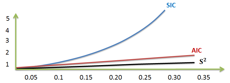 Consistency
The consistency of a model selection criteria is the key property in its evaluation. The following are some of the conditions that are to be for a model selection criteria to be consistent:
Question 1
A trend model has the following characteristics:
Let’s define the “corrected MSE” as the MSE that is penalized for degrees of freedom used.
Compute the (i) the mean squared error (MSE), (ii) the corrected MSE, and (iii) the standard error of the regression (SER).
The correct answer is C.
$$ MSE=\frac { SSR }{ T } = \frac { 785 }{ 60 } = 13.08 $$
$$ Corrected \quad MSE=\frac { SSR }{ T – k } = \frac { 785 }{ 60 – 6 } = 14.54 $$
$$ SER = \sqrt{Corrected \quad MSE} = \sqrt { \frac { SSR }{ T – k } } = \sqrt { \frac { 785 }{ 60 – 6 } } = 3.813 $$
Offered by AnalystPrep


Get Ahead on Your Study Prep This Cyber Monday! Save 35% on all CFA® and FRM® Unlimited Packages. Use code CYBERMONDAY at checkout. Offer ends Dec 1st.