Random Variables

After completing this reading, you should be able to:

• Describe and distinguish a probability mass function from a cumulative distribution function and explain the relationship between these two.
• Understand and apply the concept of a mathematical expectation of a random variable.
• Describe the four common population moments.
• Explain the differences between a probability mass function and a probability density function.
• Characterize the quantile function and quantile-based estimators.
• Explain the effect of a linear transformation of a random variable on the mean, variance, standard deviation, skewness, kurtosis, median, and interquartile range.

Random Variables

A random variable is a variable whose possible values are outcomes of a random phenomenon. It is a function that maps outcomes of a random process to real values. It can also be termed as the realization of a random process.

Precisely, if \(\omega \) is an element of a sample space Ω and x is the realization, then \(X(\omega) = x\). Conventionally, random variables are given in upper case (such as X, Y, and Z) while the realized random values are represented in lower case (such as x, y, and z)

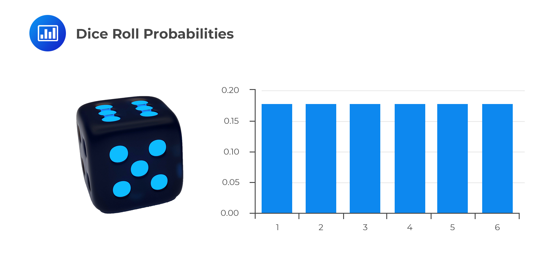
For example, let X be the random variable as a result of rolling a die. Therefore, x is the outcome of one roll, and it could take any of the values 1, 2, 3, 4, 5, or 6. The probability that the resulting random variable is equal to 3 can be expressed as:

$$ P(X = x) \text{ where } x = 3$$

Types of Random Variables

Discrete Random Variables

A discrete random variable is one that produces a set of distinct values. A discrete random variable manifests:

• If the range of all possible values is a finite set, e.g., {1,2,3,4,5,6} as in the case of a six-sided die or,
• If the range of all possible values is a countably infinite set: e.g. {1,2,3, … }

Examples of discrete random variables include:

• Picking a random stock from the S&P 500.
• The number of candidates registered for the FRM level 1 exam at any given time.
• The number of study topics in a program.

Probability Functions under Discrete Random Variables

Since the possible values of a random variable are mostly numerical, they can be explained using mathematical functions. A function \(f_X (x)=P(X=x)\) for each x in the range of X is the probability function (PF) of X and explains how the total chance (which is 1) is distributed amongst the possible values of X.

There are two functions used when explaining the features of the distribution of discrete random variables: probability mass function (PMF) and cumulative distribution function (CDF).

Probability Mass Function (PMF)

This function gives the probability that a random variable takes a particular value. Since PMF outputs the probabilities, it should possess the following properties:

1. \(f_X (x) \ge 0 \quad \forall \text{ range of X }\)(value returned must be a nonnegative)
2. \(\sum_x f_X (x)=1 \) (sum across all value in support of a random variable should be equal to 1)

Example: Bernoulli Distribution

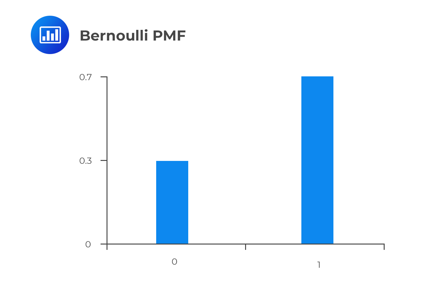
Assume that X is a Bernoulli random variable, the PMF of X is given by:

$$ f_X (x)=p^x (1-p)^{1-x},X=0,1 $$

The Random variables in a Bernoulli distribution are 0 and 1. Therefore,

$$ f_X (0)=p^0 (1-p)^{1-0}=1-p $$ And $$ f_X (1)=p^1 (1-p)^{1-1}=p $$ Looking at the above results, the first property \(f_X (x) \ge 0)\) of probability distributions is met. For the second property: $$ \sum_x f_X (x)= \sum_{x=0,1} f_X (x)=1-p+ p=1 $$ Moreover, the probability that we observe random variable 0 is 1-p, and the probability of observing random variable 1 is p. More precisely,

$$ F_X (x)=\begin{cases} 1-p,&x=0 \\ p,&x=1   \end{cases} $$

The graph of the Bernoulli PMF is shown below, assuming the p=0.7. Note that PMF is only defined for X=0,1. 

Cumulative Distribution Function (CDF)

CDF measures the probability of realizing a value less than or equal to the input x, \(Pr⁡(X \le x)\). It is denoted by \(F_X (x)\) and so,

$$ F_X (x)=Pr⁡(X \le x) $$ CDF is monotonic and increasing in x since it measures total probability. It is a continuous function (in contrast with PMF) because it supports any value between 0 and 1 (in the case of Bernoulli random variables) inclusively.

For instance, the CDF of the Bernoulli random variable is:

$$ F_X (x)=\begin{cases} 0,&x<0 \\ 1-p,&0≤x<1 \\ 1,&x\ge1  \end{cases} $$

\(F_X (x)\) is defined for all real values of x. The graph of \(F_X (x)\) against x begins at 0 then rises by jumps as values of x are realized for which p(X = x) is positive. The graph reaches its maximum value at 1. For the Bernoulli distribution with p=0.7, the graph is shown below: 

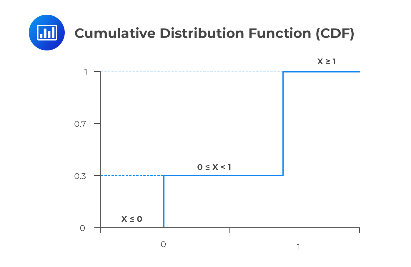Since CDF is defined for all values of x, the CDF for a Bernoulli distribution with a parameter p=0.7 is:
$$ F_X (x)=\begin{cases} 0,&x<0 \\ 0.3,&0≤x<1 \\ 1,&x\ge1  \end{cases} $$

 The corresponding graph is as shown above

Relationship Between the CDF and PMF with Discrete Random Variables

The CDF can be represented as the sum of the PMF for all the values that are less than or equal to x. Simply put:

$$ F_X (x)=\sum_{t \epsilon R(x),t \le x} f_X (t) $$ Where R(x) is the range of realized values of X (X=x).

On the other hand, PMF is equivalent to the difference between the consecutive values of X. That is:

$$ f_X (x)=F_X (x)-F_X (x-1) $$

Example: PMF and CDF under Discrete Random Variables

There are 8 hens with different weights in a cage. Hens1 to 3 weigh 1 kg, hens 4 and 5 weigh 2kg, and the rest weigh 3kg. We need to develop the PMF and the CDF.

Solution

The random variables (X = 1kg, 2kg, or 3kg) here are the weights of the chicken,

$$ \begin{align*} f_X (1) & =Pr(X=1)=\cfrac {3}{8} \\ f_X (2) & =Pr(X=2)=\cfrac {2}{8}=\cfrac {1}{4} \\ f_X (3) & =Pr(X=3)=\cfrac {3}{8} \\ \end{align*} $$ So, the PMF is: $$ \begin{cases} \frac { 3 }{ 8 } , & x=1 \\ \frac { 1 }{ 4 } , & x=2 \\ \frac { 3 }{ 8 } , & x=3 \end{cases} $$ For the CDF, it includes all the realized values of the random variable. So, $$ \begin{align*} F_X (0) & =Pr⁡(X \le 0)=0 \\ F_X (1) & =Pr⁡(X \le 1)=\cfrac {3}{8} \\ F_X (2) & =Pr⁡(X \le 2)=\cfrac {3}{8}+\cfrac {2}{8}=\cfrac {5}{8} \left[ \text{Using } F_X (x)=\sum_{t \epsilon R(x),t \le x} f_X (t) \right] \\ F_X (3) & =Pr⁡(X \le 3)=\cfrac {5}{8}+\cfrac {3}{8}=1 \\ \end{align*} $$ So that the CDF is $$ F_X (x)=\begin{cases} 0, & x < 1 \\ \frac { 3 }{ 8 } , & 1\le x < 2 \\ \frac { 5 }{ 8 } , & 2\le x < 3 \\ 1, & 3 \le x \end{cases} $$ Note that $$ f_X (x)=F_X (x)-F_X (x-1) $$ Which implies that: $$ f_X (3)=F_X (3)-F_X (2)=1-\cfrac {5}{8}=\cfrac {3}{8} $$ Which gives the same result as before.

Continuous Random Variables

A continuous random variable can assume any value along a given interval of a number line. For instance, \(x > 0,(-\infty < x < \infty ) \text{ and } 0 < x < 1\). Examples of continuous random variables include the price of stock or bond, or the value at risk of a portfolio at a particular point in time.

The following relationship holds for a continuous random variable X:

$$ P[r_1 < X < r_2 ]=p $$ This implies that p is the likelihood that the random variable X falls between \(r_1\) and \(r_2\).

The Probability Density Function (PDF) under Continuous Random Variables

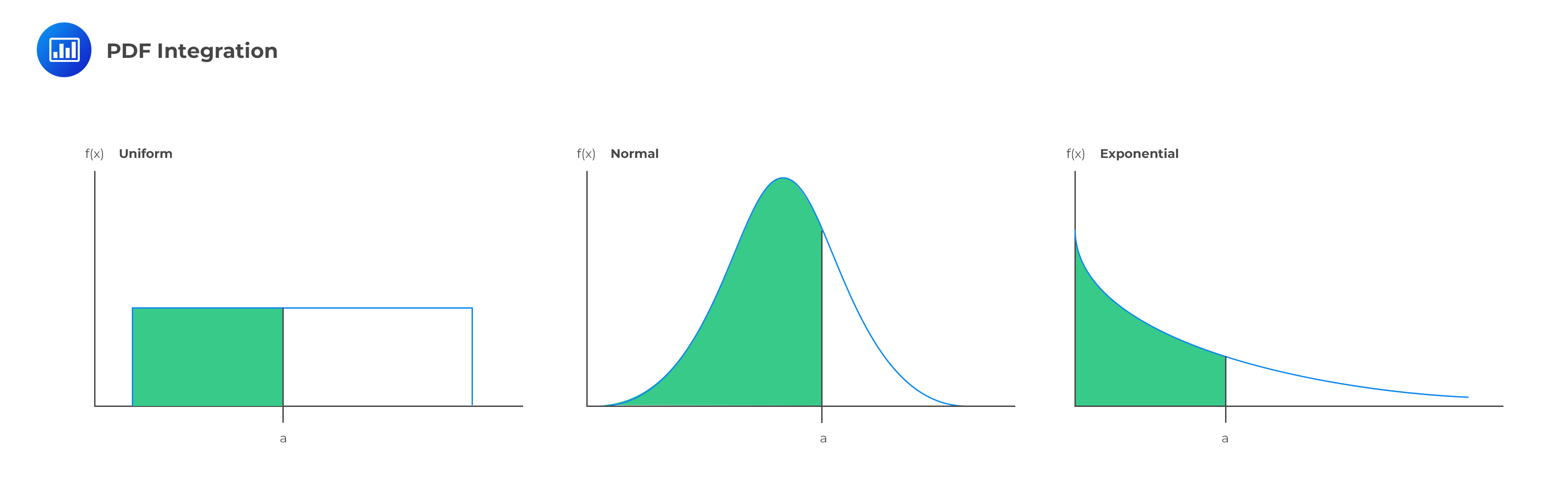
A probability density function (PDF) allows us to calculate the probability of an event.

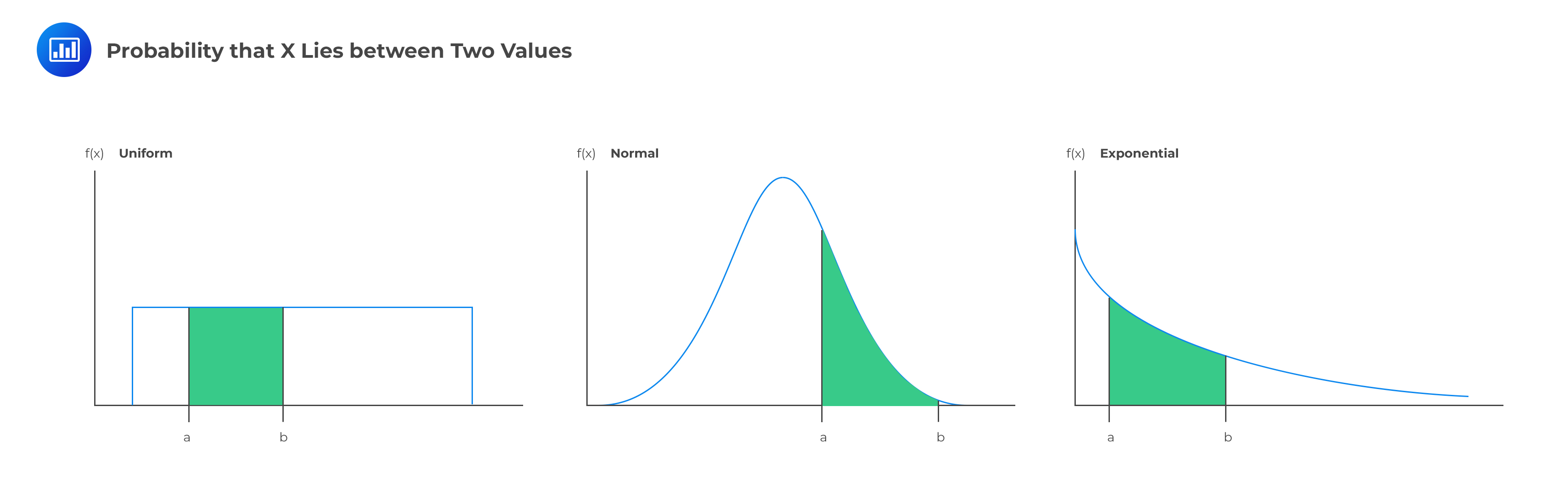
Given a PDF f(x), we can determine the probability that x falls between a and b:

$$ Pr⁡(a < x \le b)=\int _{ a }^{ b }{ f\left( x \right) dx } $$ The probability that X lies between two values is the area under the density function graph between the two values: 

Probability distribution function is another term used to refer to the probability density function. The properties of the PDF are the same as those of PMF. That is:

1. \(f_X (x) \ge 0,-\infty \le x \le \infty\) (nonnegativity)
2. \(\int_{r_{min}}^{r_{max}} f(x)dx=1\)(The sum of all probabilities must be equal to 1, just like in discrete random variables)

The upper and lower bounds of f(x) are defined by \(r_{min}\) and \(r_{max}\)

Cumulative Distribution Functions (CDF) under Continuous Random Variables

It is also called the cumulative density function and is closely related to the concept of a PDF. CDFA CDF defines the likelihood of a random variable falling below a specific value. To determine the CDF, the PDF is integrated from its lower bound.

The corresponding density function’s capital letter has traditionally been used to denote the CDF. The following computation depicts a CDF, F(x), of a random variable X whose PDF is f(x):

$$ F(a)=\int_{-\infty}^{a}f(x)d(x) =P[X \le a] $$ The region under the PDF is a depiction of the CDF. The CDF is usually non-decreasing and varies from zero to one. We must have a zero CDF at the minimum value of the PDF. The variable cannot be less than the minimum. The likelihood of the random variable is less than or equal to the maximum is 100%.

To obtain the PDF from the CDF, we have to compute the first derivative of the CDF. Therefore:

$$ f(x)=\cfrac {dF(x)}{dx} $$ Next, we look at how to determine the probability that a random variable X will fall between some two values, a and b. $$ P[a < X \le b]=\int_a^b f(x)dx=F(b)-F(a) $$ Where a is less than b.

The following relationship is also true:

$$ P[X > a]=1-F(a) $$

Example:Formulating the CDF of a Continuous Random Variable

The continuous random variable X has a pdf of \(f(x)=12x^2 (1-x) \text{ for } 0 < x < 1\). We need to find the expression for F(x).

Solution

We know that: $$ \begin{align*} F(x) & =\int_{-\infty }^x f(t)d(t) \\ F(x) & =\int_0^x 12t^{2} (1-t)d(t)={ [4t^3-3t^4 ] }_{ 0 }^{ x }=x^3 (4-3x) \end{align*} $$ So, $$ F(x)=x^3 (4-3x) $$

Expected Values

The expected values are the numerical summaries of features of the distribution of random variables. Denoted by E[X] or \(\mu\), it gives the value of X that is the measure of average or center of the distribution of X. The expected value is the mean of the distribution of X.

For discrete random variables, the expected value is given by: $$ E[X]=\sum_x xf(X) $$ It is simply the sum of the product of the value of the random variable and the probability assumed by the corresponding random variable.

Example: Calculating the Expected Value in Discrete Random Variable

There are 8 hens with different weights in a cage. Hens 1 to 3 weigh 1 kg, hens 4 and 5 weigh 2kg, and the rest weigh 3kg. We need to calculate the mean weight of the hens.

Solution

We had calculated the PDF as: $$ f(x)=\begin{cases} \frac { 3 }{ 8 } , & x=1 \\ \frac { 1 }{ 4 } , & x=2 \\ \frac { 3 }{ 8 } , & x=3 \end{cases} $$ Now, $$ E[X]=\sum_x xf(X)=1×\frac {3}{8}+2×\frac {1}{4}+3×\frac {3}{8}=2 $$ So, the mean weight of the hens in the cage is 2kg.

For the continuous random variable, the mean is given by:

$$ E[X]=\int_{-\infty}^\infty xf(x)dx $$ Basically, it is all about integrating the product of the value of the random variable and the probability assumed by the corresponding random variable.

Example: Calculating the Expected Value of a Continuous Random Variable

The continuous random variable X has a pdf of \(f(x)=12x^2 (1-x)\) for \(0 < x < 1\).

We need to calculate E[X].

Solution

We know that: $$ E[X]=\int_{-\infty}^\infty xf(x)dx $$ So, $$ E(X)=\int_0^1 x12x^2 (1-x)d(x)={[3x^4-\frac{12}{5}x^5 ]}^{1}_{0}=0.6 $$ For random variables that are functions, we apply the same method as that of a “single” random variable. That is, summing or integrating the product of the value of the random variable function and the probability assumed by the corresponding random variable function.

Assume that the random variable function is g(x). Then:

$$ E[g(x)]=\sum_x g(x)f(x) $$ for the discrete case and $$ E[g(x)]=\int_{-\infty}^\infty g(x)f(x)dx $$ for the continuous case.

Example: Calculating the Expected Values Involving Functions as Random Variable.

A random variable X has PDF of: $$ f_X (x)=\frac {1}{5} x^2,\text{ for } 0 < x < 3 $$ Calculate \(E(2X+1)\)

Solution

$$ \begin{align*} E[g(x)] & =\int_{-\infty}^\infty g(x)f(x)dx \\ & =\int_{-\infty}^\infty \frac {1}{5} (2x+1) x^2 dx=\frac {1}{5} {\left[\frac {x^4}{2}+\frac {x^3}{3} \right]}^{3}_{0}=9.9 \\ \end{align*} $$

Properties of Expectation 

The expectation operator is a linear operator. Consequently, the expectation of a constant is a constant. That is, E(c)=c. Moreover, the expected value of a random variable is a constant and not a random variable.

For non-linear function g(x),E(g(x))\(\neq\) g(E(x)). For instance, \(E \left(\frac {1}{X}\right) \neq \frac {1}{E(X)} \)

The Variance of a Random Variable

The variance of random variable measures the spread (dispersion or variability) of the distribution about its mean. Mathematically,

$$ Var(X)=E(X^2 )-{E(X)}^2=E[{X-E(X)}]^2 $$ Intuitively, the standard deviation is the square root of the variance. Now, denoting \(E(X)=\mu\), then: $$ Var(X)=E(X^2 )-\mu^2 $$

Example: Calculating the Variance of Random Variable

The continuous random variable X has a pdf of \(f(x)=12x^2 (1-x)\) for \(0 < x < 1\).

We need to calculate Var[X].

Solution

We know that: $$ Var(X)=E(X^2 )-{E(X)}^2 $$ We had calculated E(X)=0.6

We have to calculate: $$E(X^2 )$$

$$ \begin{align*} E(X ) & =\int_0^1 x.[12x^2 (1-x)]dx={[3x^4-\frac{12}{5}x^5 ]}^{1}_{0}=0.6 \\ E(X^2 ) & =\int_0^1 12x^4-12x^5 dx={ \left[ \frac {12}{5} x^5-2x^6 \right] }^{1}_{0}=0.4 \\ \end{align*} $$ So, $$ Var(X)=0.4-0.6^2=0.04 $$

Moments

Moments are defined as the expected values that briefly describe the features of a distribution. The first moment is defined to be the expected value of X:

$$ \mu_1=E(X) $$ Therefore, the first moment provides the information about the average value. The second and higher moments are broadly divided into Central and Non-central moments

Central Moments

The general formula for the central moments is: $$ \mu_k=E([X-E(X)]^k ),k=2,3… $$ Where k denotes the order of the moment. Central moments are moments about the mean.

Non-Central Moments

Non-central moments describe those moments about 0. The general formula is given by: $$ \mu_k=E(X^k) $$ Note that the central moments are constructed from the non-central moments and the first central and non-central moments are equal \(( \mu_1=E(X))\).

Population Moments

The four common population moments are: mean, variance, skewness, and kurtosis.

The Mean

The mean is the first moment and is given by: $$ \mu=E(X) $$ It is the average (also called the location of the distribution) value of X.

The Variance

This is the second moment. It is presented as: $$ \sigma^2=E([X-E(X)]^2 )=E[(X-\mu)^2 ] $$ The variance measures the spread of the random variable from its mean. The standard deviation (\(\sigma\)) is the square root of the variance. The standard deviation is more commonly quoted in the world of finance because it is easily comparable to the mean since they share the measurement units.

The Skewness

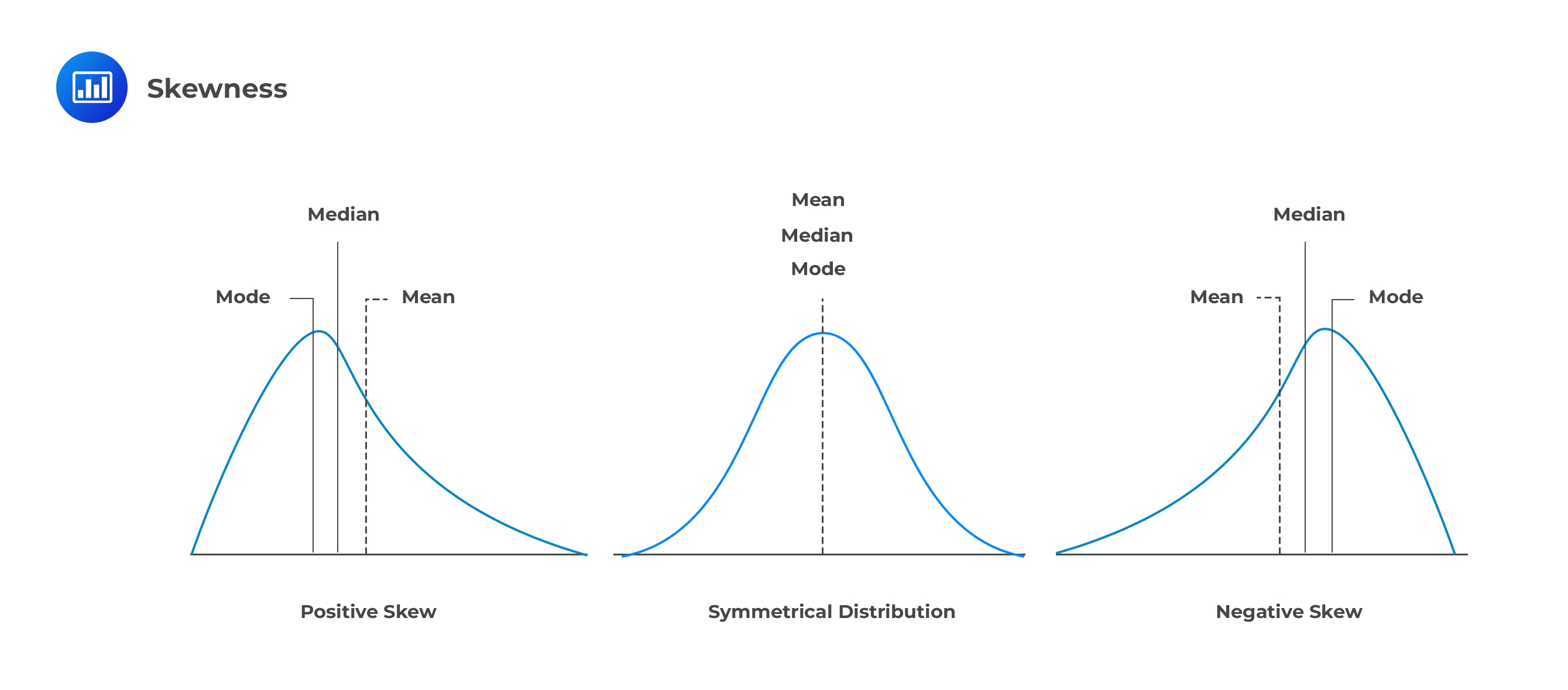
Skewness is a cubed standardized central moment given by: $$ \text{skew}(X)=\cfrac { E([X-E(X)])^3 }{\sigma^3} =E \left[ \left( \cfrac {X-\mu}{\sigma} \right)^3 \right] $$ Note that \(\cfrac {X-\mu}{\sigma}\) is a standardized X with a mean of 0 and a variance of 1.

Skewness can be positive or negative.

Positive skew

• The right tail is longer
• The mass of the distribution is concentrated on the left
• There are a few relatively high values.
• In most cases (but not always), the mean is greater than the median, or equivalently, the mean is greater than the mode; in which case the skewness is greater than zero.

Negative skew

• The left tail is longer
• The mass of the distribution is concentrated on the right
• The distribution has a few relatively low values.
• In most cases (but not always), the mean is lower than the median, or equivalently, the mean is lower than the mode, in which case the skewness is lower than zero.

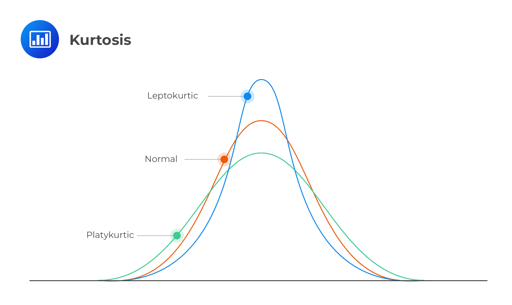
Kurtosis

The Kurtosis is defined as the fourth standardized moment given by: $$ \text{Kurt}(X)=\cfrac {E([X-E(X)]^4 }{\sigma^4} =E \left[ \left( \cfrac {X-\mu}{\sigma} \right)^4 \right] $$ The description of kurtosis is analogous to that of the Skewness only that the fourth power of the Kurtosis implies that it measures the absolute deviation of random variables. The reference value of a normally distributed random variable is 3. A random variable with Kurtosis exceeding 3 is termed to be heavily or fat-tailed.

Effect of Linear Transformation on Moments

In very basic terms, a linear transformation is a change to a variable characterized by one or more of the major math operations:

• adding a constant to the variable,
• subtracting a constant from the variable,
• multiplying the variable by a constant,
• and/or dividing the variable by a constant.

Transformation results in the formation of a new random variable.

If X is a random variable and \(\alpha\) and \(\beta\) are constants, then \(\alpha +\beta x\) is a linear transformation of X. \(\alpha\) is referred to as the shift constant, and \(\beta\) is the scale constant. The transformation shifts X by \(\alpha\) and scales it by \(\beta\). The process results in the formation of a new random variable, usually denoted by Y.

$$Y=\alpha +\beta x$$

Linear transformation of random variables is informed by the fact that many variables used in finance and risk management do not have a natural scale.

Example: Linear Transformation of Random Variables

Suppose your salary is \(\alpha\) dollars per year, and you are entitled to a bonus of \(\beta\) dollars for every dollar of sales you successfully bring in. Let X be what you sell in a certain year. How much in total do you make?

Solution

We can linearly transform the sales variable X into a new variable Y that represents the total amount made.

                                    $$Y=\alpha +\beta x$$

Where \(\alpha\) serves as the shift constant and \(\beta\)  as the scale constant.

Effect on Mean and Variance

If \(Y= \alpha + \beta x\), where \(\alpha\) and \(\beta\) are constants. The mean of Y is given by: $$ E(Y)=E(\alpha + \beta x )=\alpha + \beta E(X) $$ The variance is given by: $$ \text{Var}(Y)=\text{Var}(\alpha + \beta x)=\beta^2 \text{Var}(X)=\beta^2 \sigma^2 $$ 

The shift parameter \(\alpha\) does not affect the variance. Why? Because variance is a measure of spread from the mean; adding \(\alpha\) does not change the spread but merely shifts the distribution to the left or right.

 The standard deviation of Y is given by:

$$\sqrt { { \beta  }^{ 2 }{ \sigma  }^{ 2 } } =\left| \beta  \right| \sigma $$

It also follows that \(\alpha\) does not affect the standard deviation.

Effect on Skewness and Kurtosis

It can also be shown that if \(\beta\) is positive (so that \(Y=\alpha +\beta x\) is an increasing transformation), then the skewness and kurtosis of Y are identical to the skewness and kurtosis of X. This is because both moments are defined on standardized quantities, which removes the effect of the shift constant \(\alpha\) and the scaling factor \(\beta\). This can be seen as follows:

We know that:

$$ \text{skew}(X)=E \left[ \left( \cfrac {X-\mu}{\sigma} \right)^3 \right ] $$ Now, $$ \begin{align*} \text{skew}(Y) & =\cfrac {E([Y-E(Y)])^3 }{σ^3} =E \left[ \left( \cfrac {Y-E(Y)}{\sigma} \right)^3 \right] \\ & =E \left[ \left( \cfrac {\alpha + \beta X-(\alpha + \mu X)}{\beta \sigma } \right)^3 \right] \\ & =E \left[ \left( \cfrac {β(X-μ)}{βσ} \right)^3 \right]=E \left[ \left( \cfrac {X-μ}{σ} \right)^3 \right]=\text{Skew}(X) \\ \end{align*} $$

However, if \( \beta < 0 \), the magnitude of skewness of Y is the same as that of X but with the opposite sign because of the odd power (i.e., 3). On the other hand, the kurtosis is unaffected because it uses an even power (i.e., 4).

Quantiles and Modes

Just like any data, quantities such as the quantiles and the modes are used to describe the distribution.

The Quantiles

For a continuous random variable X, the \(\alpha\)-quartile of X is the smallest number m such that: $$ Pr⁡(X < m)=\alpha $$ Where \( \alpha \epsilon [0,1] \)

For instance, if X is a continuous random variable, the median is defined to be the solution of:

$$ P(X < m)=\int_{-\infty}^{m} f_X (x)dx=0.5 $$ Similarly, the lower and upper quartile is such that \(P(X < Q_1 )=0.25\) and \(P(X < Q_3 )=0.75\)

The interquartile range (IQR), is an alternative measure of spread. It is given by:

$$ \text{IQR}=Q_3-Q_1 $$

Example: Calculating the Quartiles of a PDF

The random variable X has a pdf given by:

$$ f_X (x)=3e^{-2x},x > 0 $$. Calculate the median of the distribution.

Solution

Denote the median by m. Then m is such that: $$ P(X < m)=\int_0^m 3e^{-2x} dx=0.5 $$ So, $$ \begin{align*} & ={\left[-\frac {3}{2} e^{-2x} \right]}^{m}_{0}=0.5 \\ & =-\frac {3}{2} e^{-2m}+\frac {3}{2}=0.5 \\ \Rightarrow m & =-\frac {1}{2}×ln⁡ \frac {2}{3}=0.2027 \\ \end{align*} $$

Mode

The mode measures the common tendency, that is, the location of the most observed value of a random variable. In a continuous random variable, the mode is represented by the highest point in the PDF.

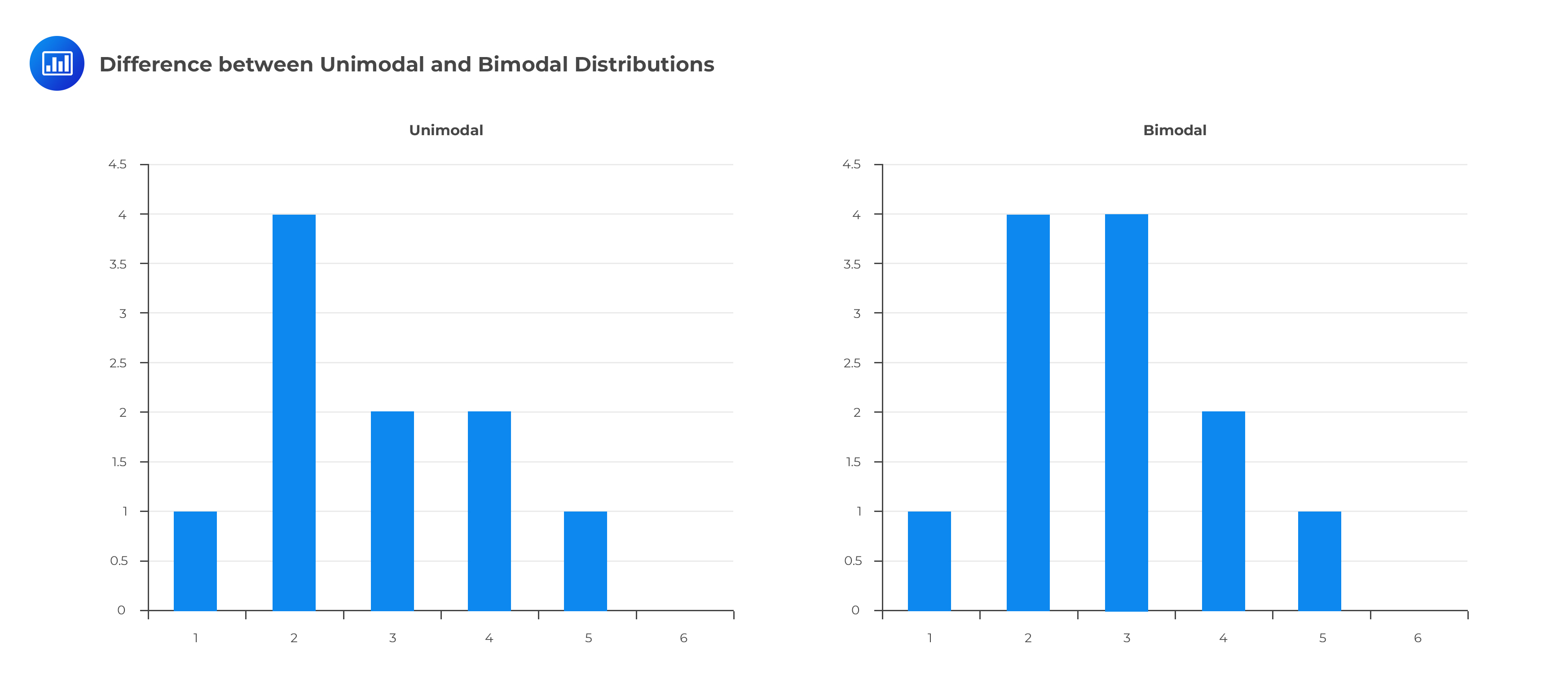
Random variables can be unimodal if there’s just one mode, bimodal if there are two modes, or multimodal if there are more than two modes.

The graph below shows the difference between unimodal and bimodal distributions.

Question 1

If a random variable \(X\) has a mean of 4 and a standard deviation of 2, calculate Var(3 – 4x)

A. 29

B. 30

C. 64

D. 35

Solution

The correct answer is C.

Recall that: $$ \text{Var}(\alpha+ \beta x)=\beta^2 \text{Var}(Y) $$ So, $$ \text{Var}(3-4X)=(-4)^2 \text{Var}(X)=16 \text{ Var}(X) $$ But we are given that the standard deviation is 2, implying that the variance is 4.

Therefore,

$$ \text{Var}(3-4X)=16×4=64 $$

Question 2

A continuous random variable has a pdf given by \(f_X (x)=ce^{-3x}\) for all \(x > 0\). Calculate Pr(X<6.5)

A. 0.4532

B. 0.4521

C. 0.3321

D. 0.9999

Solution

The correct answer is D.

We need to find the constant c first. We know that: $$ \int_{-\infty}^\infty f(x)dx=1 $$ So, $$ \begin{align*} \int_0^\infty ce^{-3x} dx & =1=c{ \left[ -\frac {1}{3} e^{-3x} \right] }^{\infty}_{0}=c \left[ 0- – \frac {1}{3} \right ] =1 \\ & \Rightarrow c=3 \\ \end{align*} $$ Therefore, the PDF is \(f_X (x)=3e^{-3x}\) so that \(Pr(X <6.5)\) is given by: $$ \begin{align*} \int_0^{6.5} 3e^{-3x} dx & =3 { \left[- \frac {1}{3} e^{-3x} \right]}^{6.5}_{0}=c \left[- \frac {1}{3} e^{-3×6.5}- – \frac {1}{3} \right] \\ & =0.9999 \\ \end{align*} $$