Fundamentals of Probability

After completing this reading, you should be able to:

• Describe an event and an event space.
• Describe independent events and mutually exclusive events.
• Explain the difference between independent events and conditionally independent events.
• Calculate the probability of an event for a discrete probability function.
• Define and calculate a conditional probability.
• Distinguish between conditional and unconditional probabilities.
• Explain and apply Bayes’ rule.

Probability is the foundation of statistics, risk management, and econometrics. Probability quantifies the likelihood that some event will occur. For instance, we could be interested in the probability that there will be a defaulter in a prime mortgage facility.

Sample Space, Event Space, and Events

Sample Space (Ω)

A sample space is defined as a collection of all possible occurrences of an experiment. The outcomes are dependent on the problem being studied. For example, when modeling returns from a portfolio, the sample space is a set of real numbers. As another example, assume we want to model defaults in loan payment; we know that there can only be two outcomes: either the firm defaults or it doesn’t. As such, the sample space is Ω = {Default, No Default}. To give yet another example, the sample space when a fair six-sided die is tossed is made of six different outcomes:

Ω = {1, 2, 3, 4, 5, 6}

Events (ω)

An event is a set of outcomes (which may contain more than one element). For example, suppose we tossed a die. A “6” would constitute an event. If we toss two dice simultaneously, a {6, 2} would constitute an event. An event that contains only one outcome is termed an elementary event. 

Event Space (F)

The event space refers to the set of all possible outcomes and combinations of outcomes. For example, consider a scenario where we toss two fair coins simultaneously. The following would constitute our event space:

{HH, HT, TH, TT}

Note: If the coins are fair, the probability of a head, P(H), equals the probability of a tail, P(T).

Probability

The probability of an event refers to the likelihood of that particular event occurring. For example, the probability of a Head when we toss a coin is 0.5, and so is the probability of a Tail.

According to frequentist interpretation, the term probability stands for the number of times an event occurs if a set of independent experiments is performed. But this is what we call the frequentist interpretation because it defines an event’s probability as the limit of its relative frequency in many trials. It is just a conceptual explanation; in finance, we deal with actual, non-experimental events such as the return earned on a stock.

Independent and Mutually Exclusive Events

Mutually Exclusive Events

Two events, A and B, are said to be mutually exclusive if the occurrence of A rules out the occurrence of B, and vice versa. For example, a car cannot turn left and turn right at the same time.

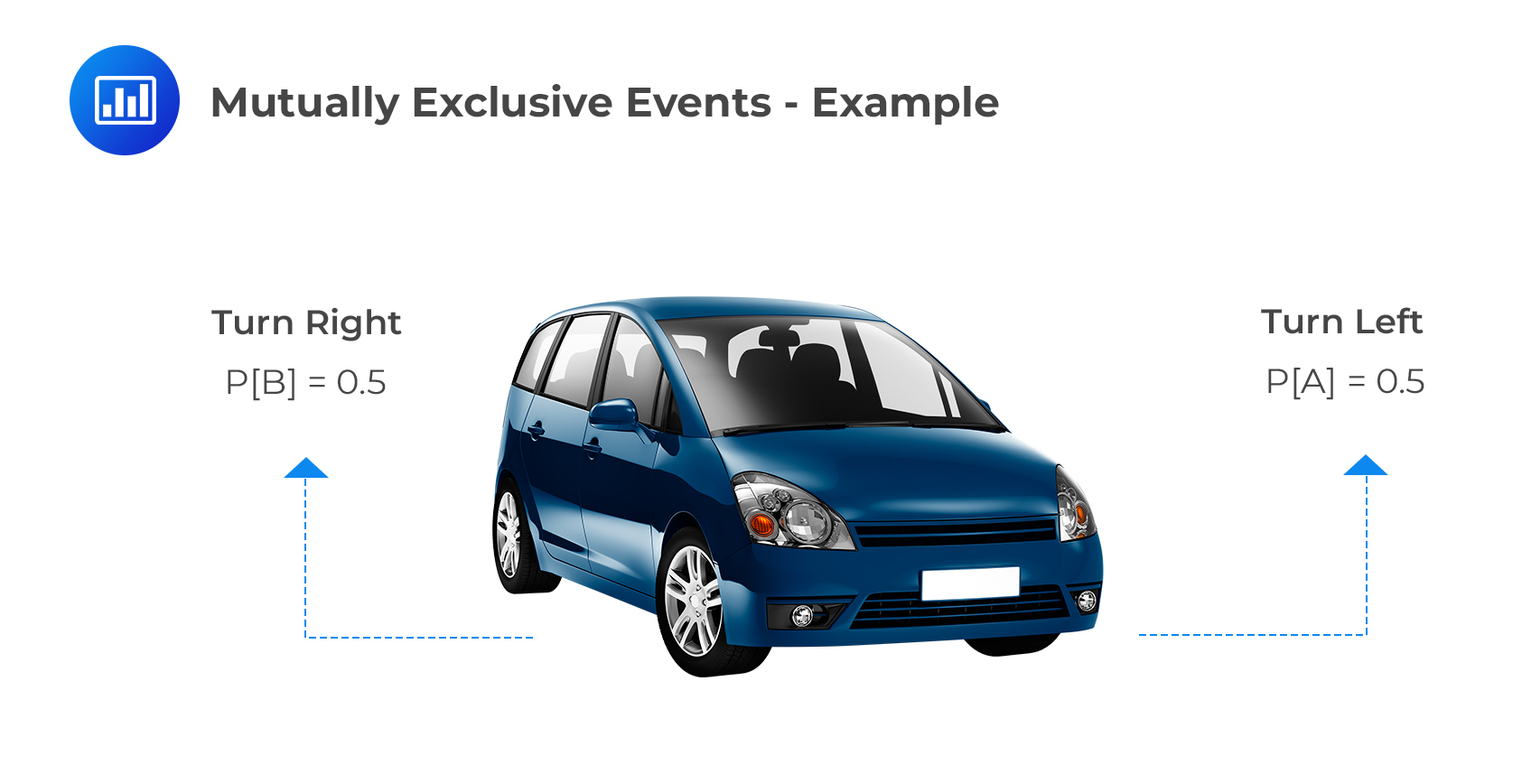
Mutually exclusive events are such that one event precludes the occurrence of all the other events. Thus, if you roll a dice and a 4 comes up, that particular event precludes all the other events, i.e., 1,2,3,5 and 6. In other words, rolling a 1 and a 5 are mutually exclusive events: they cannot occur simultaneously.

Furthermore, there is no way a single investment can have more than one arithmetic mean return. Thus, arithmetic returns of, say, 20% and 17%  constitute mutually exclusive events.

Independent Events

Two events, A and B, are independent if the fact that A occurs does not affect the probability of B occurring. When two events are independent, this simply means that both events can happen at the same time. In other words, the probability of one event happening does not depend on whether the other event occurs or not. For example, we can define A as the likelihood that it rains on March 15 in New York and B as the probability that it rains in Frankfurt on March 15. In this instance, both events can happen simultaneously or not.

Another example would be defining event A as getting tails on the first coin toss and B on the second coin toss. The fact of landing on tails on the first toss will not affect the probability of getting tails on the second toss.

Intersection

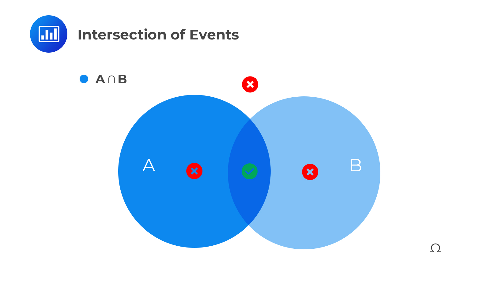
The intersection of events say A and B is the set of outcomes occurring both in A and B. It is denoted as P(A∩B). Using the Venn diagram, this is represented as:

For independent events,

$$P(A∩B)=P(A \text{ and } B)=P(A)×P(B)$$

Independence can be extended to n independent events: Let \(A_1,A_2,…, A_n\) be independent events then:

$$P(A_1∩A_2∩…∩ A_n  )=P(A_1)×P(A_2 )×…×P(A_n )$$

For mutually exclusive events,

$$P(A∩B)=P(A \text{ and } B)=0$$

This is because of the occurrence of A rules out the occurrence of B. Remember that a car cannot turn left and turn right at the same time!

Union

The union of events, say, A and B, is the set of outcomes occurring in at least one of the two sets – A or B. It is denoted as P(A∪B). Using the Venn diagram, this is represented as:

To determine the likelihood of any two mutually exclusive events occurring, we sum up their individual probabilities. The following is the statistical notation:

$$ P\left( A\cup B \right) =P(A \text{ or } B)=P\left( A \right) +P\left( B \right) $$

Given two events A and B, that are not mutually exclusive (independent events), the probability that at least one of the events will occur is given by:

$$P(A \cup B)=P(A \text{ or } B) = P(A)+P(B)-P(A \cap B)$$

The Complement of a Set

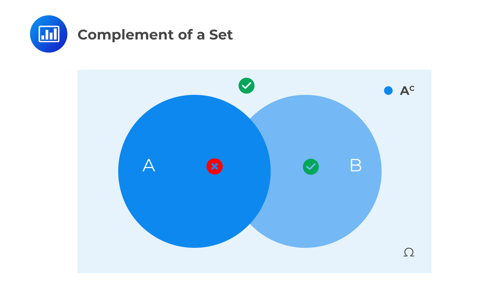
Another important concept under probability is the compliment of a set denoted by Ac (where A can be any other event) which is the set of outcomes that are not in A. For example, consider the following Venn diagram:

This is the first axiom of probability, and it implies that:

$$P(A ∪ A^c )=P(A)+P(A^c )=1$$

Conditional Probability

Until now, we’ve only looked at unconditional probabilities. An unconditional probability (also known as a marginal probability) is simply the probability that an event occurs without considering any other preceding events. In other words, unconditional probabilities are not conditioned on the occurrence of any other events; they are ‘stand-alone’ events.

Conditional probability is the probability of one event occurring with some relationship to one or more other events. Our interest lies in the probability of an event ‘A’ given that another event ‘B ‘has already occurred. Here’s what you should ask yourself:

“What is the probability of one event occurring if another event has already taken place?” We pronounce P(A | B) as “the probability of A given B.,” and it is given by:

$$P(A│B)=\frac{P(A\cap B)}{P(B)}$$

The bar sandwiched between A and B simply indicates “given.”

Bayes’ Theorem

Bayes’ theorem describes the probability of an event based on prior knowledge of conditions that might be related to the event. Assuming that we have two random variables, A and B, then according to Bayes’ theorem:

$$ P\left( A|B \right) =\frac { P\left( B|A \right) \times P\left( A \right) }{ P\left( B \right) } $$

Applying Bayes’ Theorem

Supposing that we are issued with two bonds, A and B. Each bond has a default probability of 10% over the following year. We are also told that there is a 6%  chance that both the bonds will default, an 86% chance that none of them will default, and a 14% chance that either of the bonds will default. All of this information can be summarized in a probability matrix.

Often, there is a high correlation between bond defaults. This can be attributed to the sensitivity displayed by bond issuers when dealing with broad economic bonds. The 6% chances of both the bonds defaulting are higher than the 1% chances of default had the default events been independent.

The features of the probability matrix can also be expressed in terms of conditional probabilities. For example, the likelihood that bond \(A\) will default given that \(B\) has defaulted is computed as:

$$ P\left( A|B \right) =\frac { P\left[ A\cap B \right] }{ P\left[ B \right] } =\frac { 6\% }{ 10\% } =60\% $$

This means that in 60% of the scenarios in which bond \(B\) will default, bond \(A\) will also default.

The above equation is often written as:

$$ P\left[ A\cap B \right] =P\left( A|B \right) \times P\left[ B\right] \quad \quad \quad \quad I $$

Also:

$$ P\left[ A\cap B \right] =P\left( B|A \right) \times P\left[ A \right] \quad \quad \quad \quad II $$

Both the right-hand sides of equations \(I\) and \(II\) are combined and rearranged to give the Bayes’ theorem:

$$P(B│A)×P[A]=P(A│B)×P(B)$$

$$ \Rightarrow P\left( A|B \right) =\frac { P\left( B|A \right) \times P\left[ A \right] }{ P\left[ B \right] } $$

When presented with new data, Bayes’ theorem can be applied to update beliefs. To understand how the theorem can provide a framework for how exactly the new beliefs should be, consider the following scenario:

Example: Applying Baye’s Theorem

Suppose that an analyst could group fund managers into two categories, star and non-star managers, after evaluating historical data. Given that the best managers are a star and there is a 75% likelihood that in a particular year, the market will be beaten by a star. On the other hand, there are equal chances that non-star managers will either beat the market or underperform it. Furthermore, there is year-to-year independence in the probabilities that both types of managers will beat the market.

Only 16% of managers within a given cohort become stars. Three years have passed since a new manager who was able to beat the market every single year was added to the portfolio of the analyst. Determine the chances of the manager being a star when he was first added to the portfolio. What are the chances of him being a star at present? What are his chances of beating the market in the following year, given that he has beaten it in the past three years?

Solution

We first summarize the data by introducing some notations as follows: The chances that a manager will beat the market on the condition that he is a star is:

$$ P\left( B|S \right) =0.75=\frac { 3 }{ 4 } $$

The chances of a non-star manager beating the market are:

$$ P\left( B|\bar { S } \right) =0.5=\frac { 1 }{ 2 } $$

The chances of the new manager being a star during the particular time he was added to the analyst’s portfolio are exactly the chances that any manager will be made a star, which is unconditional:

$$ P\left[ S \right] =0.16=\frac { 4 }{ 25 } $$

To evaluate the likelihood of him being a star at present, we compute the likelihood of him being a star given that he has beaten the market for three consecutive years, \(P\left( S|3B \right) \), using the Bayes’ theorem:

$$ P\left( S|3B \right) =\frac { P\left( 3B|S \right) \times P\left[ S \right] }{ P\left[ 3B \right] } $$

$$ P\left( 3B|S \right) ={ \left( \frac { 3 }{ 4 } \right) }^{ 3 }=\frac { 27 }{ 64 } $$

The unconditional chances that the manager will beat the market for three years is the denominator.

$$ P\left[ 3B \right] =P\left( 3B|S \right) \times P\left[ S \right] +P\left( 3B|\bar { S } \right) \times P\left[ \bar { S } \right] $$

$$ P\left[ 3B \right] ={ \left( \frac { 3 }{ 4 } \right) }^{ 3 }\times \frac { 4 }{ 25 } +{ \left( \frac { 1 }{ 2 } \right) }^{ 3 }\frac { 21 }{ 25 } =\frac { 69 }{ 400 } $$

Therefore:

$$ P\left( S|3B \right) =\frac { \left( \frac { 27 }{ 64 } \right) \left( \frac { 4 }{ 25 } \right) }{ \left( \frac { 69 }{ 400 } \right) } =\frac { 9 }{ 23 } =39\% $$

Therefore, there is a 39% chance that the manager will be a star after beating the market for three consecutive years, which happens to be our new belief and is a significant improvement from our old belief, which was 16%.

Finally, we compute the manager’s chances of beating the market the following year. This happens to be the summation of the chances of a star beating the market and the chances of a non-star beating the market, weighted by the new belief:

$$ P\left[ B \right] =P\left( B|S \right) \times P\left[ S \right] +P\left( B|\bar { S } \right) \times P\left[ \bar { S } \right] $$

$$ P\left[ B \right] =\frac { 3 }{ 4 } \times \frac { 9 }{ 23 } +\frac { 1 }{ 2 } \times \frac { 14 }{ 23 } =60\%=\frac { 3 }{ 5 } $$

We also have that:

$$ P\left( S|3B \right) =\frac { P\left( 3B|S \right) \times P\left[ S \right] }{ P\left[ 3B \right] } $$

The L.H.S of the formula is posterior. The first item on the numerator is the likelihood, and the second part is prior.

Question 1

The probability that the Eurozone economy will grow this year is 18%, and the probability that the European Central Bank (ECB) will loosen its monetary policy is 52%.

Assume that the joint probability that the Eurozone economy will grow and the ECB will loosen its monetary policy is 45%. What is the probability that either the Eurozone economy will grow or the ECB will loosen its monetary policy?

A. 42.12%

B. 25%

C. 11%

D. 17%

The correct answer is B.

The addition rule of probability is used to solve this question:
P(E) = 0.18 (the probability that the Eurozone economy will grow is 18%)
p(M) = 0.52 (the probability that the ECB will loosen the monetary policy is 52%)
p(EM) = 0.45 (the joint probability that Eurozone economy will grow and the ECB will loosen its monetary policy is 45%)

The probability that either the Eurozone economy will grow or the central bank will loosen its the monetary policy:
p(E or M) = p(E) + p(M) – p(EM) = 0.18 + 0.52 – 0.45 = 0.25

Question 2

A mathematician has given you the following conditional probabilities:

$$\begin{array}{l|l} \text{p(O|T) = 0.62} & \text{Conditional probability of reaching } \\
\text{} & \text{ the office if the train arrives on time} \\\hline
\text{p(O|T c) = 0.47} & \text{Conditional probability of reaching the office} \\
\text{} & \text{ if the train does not arrive on time} \\ \hline
\text{p(T) = 0.65} & \text{Unconditional probability of } \\
\text{ } & \text{the train arriving on time } \\ \hline
\text{p(O) = ?} & \text{Unconditional probability}\\
\text{} & \text{of reaching the office}\\ \end{array}$$

What is the unconditional probability of reaching the office, p(O)?

A. 0.4325

B. 0.5675

C. 0.3856

D. 0.5244

The correct answer is B.

This question can be solved using the total probability rule.

If p(T) = 0.65 (Unconditional probability of train arriving on time is 0.65), then the unconditional probability of the train not arriving on time p(T c) = 1 – p(T) = 1 – 0.65 = 0.35.

Now, we can solve for

$$\begin{align*}p(O)&= p(O|T) * p(T) + p(O|T c) * p(T c)\\& = 0.62 * 0.65 + 0.47 * 0.35 \\&= 0.5675\end{align*}$$

Note: p(O) is the unconditional probability of reaching the office. It is simply the addition of:

1. reaching the office if the train arrives on time, multiplied by the train arriving on time, and
2. reaching the office if the train does not arrive on time, multiplied by the train not arriving on time (or given the information, one minus the train arriving on time)

Question 3

Suppose you are an equity analyst for the XYZ investment bank. You use historical data to categorize the managers as excellent or average. Excellent managers outperform the market 70% of the time and average managers outperform the market only 40% of the time. Furthermore, 20% of all fund managers are excellent managers and 80% are simply average. The probability of a manager outperforming the market in any given year is independent of their performance in any other year.

A new fund manager started three years ago and outperformed the market all three years. What’s the probability that the manager is excellent?

A. 29.53%

B. 12.56%

C. 57.26%

D. 30.21%

The correct answer is C.

The best way to visualize this problem is to start off with a probability matrix:

$$\small{ \begin{array}{l|c|c} \textbf{Kind of manager} & \textbf{Probability} & \textbf{Probability of beating market} \\
\hline \text{Excellent} & {0.2} & {0.7}\\ \hline \text{Average} & {0.8} & {0.4}\\ \end{array}}$$

Let E be the event of an excellent manager, and A represent the event of an average manager.
P(E) = 0.2 and P(A) = 0.8

Further, let O be the event of outperforming the market.

We know that:

P(O|E) = 0.7 and P(O|A) = 0.4

We want P(E|O):

$$\begin{align*}P\left( E|O \right)&=\frac {P\left( O|E \right) \times P(E)}{ P\left( O|E \right) \times P(E) + P\left( O|A \right) \times  P(A) } \\&=\frac {\left( 0.7^{ 3 }\right) \times 0.2}{ \left( 0.7^{ 3 }\right) \times 0.2 + \left( 0.4^{ 3 }\right) \times 0.8 }\\& = 57.26 \% \end{align*}$$

Note: The power of three is used to indicate three consecutive years.