Risk Measurement and Assessment

After completing this reading, you should be able to:

• Explain best practices for the collection of operational loss data and reporting of operational loss incidents, including regulatory expectations.
• Explain operational risk-assessment processes and tools, including risk control self-assessments (RCSAs), likelihood assessment scales, and heatmaps.
• Describe the differences among key risk indicators (KRIs), key performance indicators (KPIs), and key control Indicators (KCIs).
• Describe the use of factor-based models that quantitatively assess operational risk, and explain the application of the Swiss cheese model and the bowtie tool.
• Estimate operational risk exposures based on the fault tree model given probability assumptions.
• Describe approaches used to determine the level of operational risk capital for economic capital purposes, including their application and limitations.
• Describe and explain the steps to ensure a strong level of operational resilience and to test the operational resilience of important business services.

Best Practices for the Collection of Operational Loss Data and Reporting of Operational Loss Incidents, Including Regulatory Expectations

Operational Loss Data (OLD) is essential for successful risk management. OLD is the information that organizations use to identify, measure, monitor, and control operational risks. Collecting and analyzing incident loss data provides important insights for scenario identification, risk assessment, and capital modeling.

Importance of Internal Incident Data

Organizations must be able to identify control breaches and weaknesses to prevent further losses and improve business performance, stability, and profitability. This is why internal incident data collection is important. Collecting the right kind of data enables organizations to identify the root causes of incidents that have occurred in the past, as well as potential incidents that could occur in the future. By understanding the details of each incident (e.g., processes/control breakdowns), organizations can design effective strategies to address them and reduce their losses over time.

Furthermore, having a good understanding of incident data helps organizations create more accurate scenarios for risk assessment purposes. This allows them to better predict how much capital they need to reserve for operational risks. Moreover, analyzing internal incident data provides valuable information regarding which areas require additional controls or improvements. This helps organizations become more efficient in managing their operations.

Value of External Loss Data

In addition to collecting internal incident data, it is also beneficial for organizations to analyze external loss data from other firms. Doing so provides rich insights into the risk exposure for other companies. Organizations can use these insights to compare their own operations against those of their peers or competitors—which helps them identify any areas that need improvement—and then design appropriate strategies accordingly. Such comparisons are especially useful when it comes to designing capital models. This is because they allow companies to benchmark against industry standards and ensure that they hold enough capital reserves relative to their peers—without over-reserving or under-reserving for risks a company faces (in comparison to its peers).

Beyond this, incident data can also play an important role when it comes to Pillar 2 capital requirements. The collection and analysis of loss data provide valuable insight into operational risk levels at a bank, allowing senior management teams to make informed decisions that help reduce their regulatory capital add-ons under Pillar 2. Ultimately, this allows banks to remain compliant with global regulations while ensuring that they are able to allocate sufficient capital where it will have the most impactful effect on their business operations. As such, comprehensive incident data collection and analysis play an important role when it comes to navigating modern financial risk management guidelines.

Regulatory Requirements Regarding Operational Risk Data Collection

Incident Data Collection Process

The incident data collection process is a key component of an effective risk management strategy. By understanding the details of each incident that occurs in your organization, you can better prepare for future incidents and make adjustments to minimize losses due to future events. Additionally, collecting incident data can help you identify any potential areas of improvement or opportunities for optimization in your current procedures. Lastly, having a complete record of past incidents allows you to review trends over time and understand the cause-and-effect relationship between different events.

The Basel Committee recommends that “a bank must have documented procedures and processes for the identification, collection, and treatment of internal loss data” (BCBS, point b).

When collecting incident data, there are several pieces of information that should be included in order to provide an accurate view of the event. This includes:

• Dates: When did it occur?
• Thresholds: What were the specific parameters used?
• Event types: Was it human error or a system failure?
• Loss amounts: How much money was lost?
• Impact types: What were the consequences?

If possible, you should also include information about any corrective actions taken or suggested solutions for similar events in the future.

Operational risk events differ from those caused by market and credit risks due to their mostly localized origins and ambiguous character. An operational risk event could be a virus, a bug, or an IT server crash that causes a disruption in operations. However, these different types of risk events cannot be labeled the same way. Events, such as a data breach and an account takeover, may seem similar, but they can have distinct impacts and require different processes to identify and mitigate them.

While market and credit risks usually follow easily identifiable external conditions, operational events change more subtly, and their effects are harder to predict. For example, imagine a bug in a digital banking app that results in delays in payment transfers for clients. Such an occurrence could have wide-reaching repercussions beyond those immediately present at the time of failure. These delayed payments can lead to customer complaints, demands for compensation from the bank, and negative reviews on social media—all of which damage the reputation of the bank’s services and mean extra costs in terms of management attention and IT resources. The identification and quantification of the impacts of such an event is less straightforward than recording a credit loss on a corporate loan or a market loss on a derivatives portfolio.

It is virtually universal that companies across all sectors utilize the same set of core data fields whenever operational incidents are reported. This allows for better internal and external benchmarking and visibility, helping the business to increase its efficiency on many levels. Although the inclusion of more data fields can add to a comprehensive understanding of any given incident, it also poses several risks. Too much information can lead to reporting and analysis overload as well as excessive use of resources. As such, it is best practice to include only the most essential data points and avoid overcomplicating the intake process. Furthermore, efforts should be made to consolidate these fields wherever possible in order to reduce any extra strain on staff or systems.

Table 1: Common Useful Fields in Operational Risk Incident Reporting

$$\begin{array}{|l}
\textbf{Unique Incident ID} \\ \hline
\text{Place of occurrence (business unit/division)} \\
\text{Event type (level 1, level 2)} \\
\text{Event title and description (as standardized as possible)} \\
\text{Cause type (level 1, level 2)} \\
\text{Controls that failed} \\
\text{Dates of occurrence/discovery/reporting/settlement} \\
\text{Expected direct financial loss (may evolve until closure)} \\
\text{Impact type: loss/gain/near miss} \\
\text{Indirect effects (per type): often on a scale} \\
\text{Recovery (insurance and other recoveries)} \\
\text{Net loss (gross loss minus recovery)} \\
\text{Actions plans (when appropriate): measures, owner, time schedule} \\ \text{Link with other incidents (if any)—for grouped losses and reporting} \\ \text{Other comments if necessary}
\end{array}$$

Comprehensive Data

The Basel Committee on Banking Supervision, or BCBS, requires banks to have comprehensive internal loss data, capturing all material activities and exposures in all their appropriate subsystems and geographic locations. The committee has set a minimum threshold for loss reporting at €20,000 (about $22,000). Unfortunately, the committee does not clearly define what constitutes “material” activities or exposures. Due to this, many firms set their own reporting thresholds at or below €20,000 (about $22,000). This has led to the practice of setting reporting thresholds at zero to capture every operational loss or simplify instructions to the business units that do not need to estimate a loss before deciding to report incidents. While this strategy may have an appeal in its simplicity, it is fading away among large banking institutions because of the sheer number of small incidents that must be reported with little information value gained in return. Instead, most banks and insurance companies prefer a threshold slightly lower than the regulatory limit. Thresholds of €20,000, €10,000, or €5,000 are common.

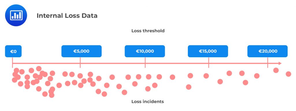
Regulatory guidelines dictate that firms must report any incidents causing them financial losses. But from a management perspective, it’s also good practice to record the non-financial impacts associated with any material operational risk events. This includes reputational damage, customer detriment, disruption of service, and use of management time and attention. While these events may not seem to have an immediate financial cost associated with them, they can often lead to costly consequences down the line. Regulatory scrutiny or customer dissatisfaction can both put major strains on a firm’s resources, while remediation plans or increased management attention can be expensive investments in the future. Ultimately, when these non-financial impacts are ignored and not properly taken into account alongside financial costs, the true cost of operational risk and poor performance can be significantly underestimated.

It is important to remember that both direct and indirect losses must be reported. Direct losses are the ones incurred immediately after the event: for example, the cost of remediation, any financial outcomes due to illegal transactions, or compensation to clients. Indirect losses are much trickier to identify since they stem from further consequences of an operational risk event. These could include customer attrition, low employee morale and productivity levels, compliance costs resulting from regulatory scrutiny, and increased insurance premiums following claims. It is important that organizations set up a reliable system by which they thoroughly capture indirect losses, often by assigning them a 1-4 impact rating based on the established Impact Assessment Matrix.

Grouped losses are an important concept in operational risk management, as they provide strong evidence that one root cause can lead to multiple geopolitical, financial, and legal consequences, each of which must be understood and addressed. Grouped losses are defined as distinct operational risks connected to a single core event or cause. For example, if an IT failure occurs, impacting various departments in different ways, this sequence of events would likely constitute one grouped loss. Similarly, if the same wrong advice were provided to numerous customers leading to a series of compensation claims, it would also meet the criteria of a grouped loss. Regulators require actuaries and other financial risk analysts to group losses to ensure the real underlying cause is correctly reflected on risk models and management reporting.

Dates of Incidents and Settlement Lags

Banks are required to report not only gross loss amounts associated with each operational loss event but also the reference dates of the event.

Each operational incident has four important dates:

• Date of occurrence: When did the event first happen?
• Date of discovery: When was it first identified?
• Date of reporting: When did it enter the reporting database?
• Date of accounting: When did the financial impact enter the general ledger?

The time gap between each pair of dates provides interesting insight. For example, the time gap between occurrence and discovery is indicative of an organization’s visibility into issues on its operations side. On top of that, the difference between discovery and reporting provides insight into how diligently incidents are reported to the risk function – an important step for mitigating risk exposure. Regulations do not require a specific date type for internal risk reporting purposes, leaving organizations to apply their policies. Generally speaking, organizations should consider a risk-based approach rather than rushing to log immaterial events, which could end up wasting resources. It’s generally accepted that material incidents should be reported within a few working days. On the other hand, minor incidents can simply be included in periodic summary reporting.

Lags in even materialization can be quite revealing. Many of the large losses that appear on accounts can be attributed to events or accumulated risk exposures that occurred several months or even years earlier. Consequently, management should duly consider the implications of this lag when modeling future operational events.

Boundary Event Reporting

Given the variety of operational losses that bankers and financial institutions must address, the Basel Committee has provided helpful guidance on the best way to classify events, particularly with respect to boundary event reporting. The boundaries it has established are particularly important to those events related to credit risk. Such incidents should only be accounted for in the lost dataset if they are not already recorded in credit risk-weighted assets (RWA). Meanwhile, operational losses related to market risk criteria must always be treated as an operational risk when calculating minimum regulatory capital.

Boundary events are occurrences that arise in a different risk category compared to their cause. For example, a credit loss may be aggravated by the incorrect recording of collateral, while a market loss could arise from an unintentional mistake when booking a position. International regulators have adopted the pragmatic view of not separating the exact cause of these boundary events. After all, credit risk models for capital requirements are based on simply capturing past losses in whatever way they occurred. So, even if operational risk caused those losses, they are still covered under credit risk and deemed acceptable from a regulatory viewpoint. This approach has allowed financial firms to avoid spending time dissecting each event and instead focus on addressing potential problems head-on while utilizing existing regulations.

Data Quality Requirements

According to the Basel Committee on Banking Supervision (BCBS), banks must initiate processes to independently review their loss data collection to ensure its comprehensiveness and accuracy. While a good starting point may be to simply track losses associated with daily operations, other sources should also be taken into account if the bank wishes to assess the depth and range of its data. Reconciling loss data with information from general ledger accounts, IT logs, and other records can help to provide insight into any potential material losses that may have been overlooked or under-reported. Though this process involves some work upfront in developing adequate systems for capturing and collating reportable losses, it ensures compliance with BCBS regulations and provides valuable insights for informed decision-making.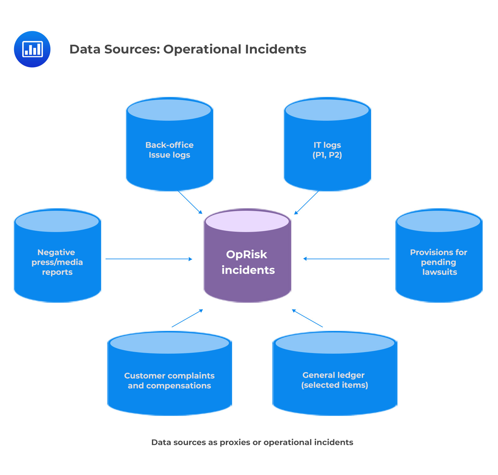

Operational Risk-assessment Processes and Tools

Risk Control Self-Assessments (RCSAs)

Risk and control self-assessment (RCSA) is an ongoing cycle of risk assessment, evaluation, and management that enables organizations to identify and mitigate risks while controlling costs. It involves a systematic review of risks in an organization’s processes, products, and services, as well as assurance that its processes are adequately managed while also maintaining compliance with laws and regulations. The RCSA looks at both inherent risks and the residual risks that remain after applying existing controls in order to create a more complete picture of the operational risk they are facing. Historically, RCSAs have been conducted yearly as part of the organization’s standard risk assessment program. But due to increasing volatility and complexity in the market, some organizations are now conducting these assessments on a quarterly basis. By evaluating the likelihood and impact of risks regularly and consistently over time, businesses can better understand their risk profile and instill confidence that their operations remain safe and secure.

While useful initially, RCSA can fall prey to subjectivity, behavioral biases, limited data inputs, and inconsistencies across different departments or business units due to different assessment practices. Standardized risk descriptions and precise rating criteria must be used to achieve maximum reliability and minimum inconsistency. This ensures that each risk has undergone a consistent assessment process regardless of where it originated from, allowing for an accurate comparison of various risks across the organization.

Severity Assessment: Impact Scales

Severity assessment is an important tool for assessing the potential impact of events. Through this kind of assessment, it is possible to identify the most severe impacts that a certain event could cause. The four most common scales used to measure impact are financial, regulatory, customer, and reputation impacts. Each of these scales uses a four or five-point rating system, with the ratings ranging from very low or insignificant to catastrophic or extremely severe impacts. In addition to these traditional scales, there has been an increase in the consideration of the continuity of services as a scale due to the regulatory attention placed on resilience.

The figure below shows a sample impact scale where financial impacts are expressed in revenues or operating profit percentages rather than in monetary amounts. Similarly, customer impacts are expressed as a percentage of the client base. Expressing financial impacts in percentages rather than dollar amounts is a great way for organizations to make sure that the impact statements are applicable to departments of all sizes. For instance, while a $100,000 financial impact might not be crucial for large, successful business units, it could have a much larger and more meaningful effect on smaller departments or offices. Relative impact definitions such as this provide organizations with an easy way to scale their standards as they expand – allowing them to function efficiently across divisions regardless of different values or operational locations.

Table 2: Example of Impact Scale Definitions and Ratings

$$\small{\begin{array}{l|l|l|l|l}
\textbf{Rating} & \textbf{Financial} & {\textbf{Service}\\\textbf{Delivery}}& {\textbf{Customer}\\\textbf{Reputation}} & \textbf{Regulatory} \\\hline
\text{Extreme} & \begin{array}{@{\labelitemi\hspace{\dimexpr\labelsep+0.5\tabcolsep}}l@{}}\text{>20% of}\\\text{operating}\\\text{income}\\\text{(OI)}\end{array} & \begin{array}{@{\labelitemi\hspace{\dimexpr\labelsep+0.5\tabcolsep}}l@{}}\text{Critical}\\\text{disruption}\\\text{of service}\\\text{resulting}\\\text{in major}\\\text{impacts to}\\\text{internal}\\\text{or external}\\\text{stakeholders}\end{array} & \begin{array}{@{\labelitemi\hspace{\dimexpr\labelsep+0.5\tabcolsep}}l@{}}\text{Significant}\\\text{reputational}\\\text{impact,}\\\text{possibly}\\\text{long-lasting}\\\text{affecting the}\\\text{organization’s}\\\text{reputation}\\\text{and trust}\\\text{towards}\\\text{several groups}\\\text{of key}\\\text{stakeholders}\end{array} & \begin{array}{@{\labelitemi\hspace{\dimexpr\labelsep+0.5\tabcolsep}}l@{}}\text{Significant}\\\text{compliance}\\\text{breach,}\\\text{resulting in}\\\text{large fines}\\\text{and increased}\\\text{regulatory}\\\text{scrutiny}\end{array} \\\hline
\text{Major} & \text{>5-20% of OI} & \begin{array}{@{\labelitemi\hspace{\dimexpr\labelsep+0.5\tabcolsep}}l@{}}\text{Significant}\\\text{service}\\\text{disruption}\\\text{affecting key }\\\text{stakeholders, }\\\text{requiring the}\\\text{crisis}\\\text{management }\\\text{plan to be}\\\text{activated}\end{array} & \begin{array}{@{\labelitemi\hspace{\dimexpr\labelsep+0.5\tabcolsep}}l@{}}\text{Reputational}\\\text{impact}\\\text{affecting >5%}\\\text{of customers.}\\\text{Lasting}\\\text{impacts}\\\text{needing}\\\text{substantial}\\\text{remediation}\\\text{plans}\end{array} & \begin{array}{@{\labelitemi\hspace{\dimexpr\labelsep+0.5\tabcolsep}}l@{}}\text{Compliance}\\\text{breach}\\\text{resulting in}\\\text{regulatory}\\\text{fines leading}\\\text{to lasting}\\\text{remediation}\\\text{programs with}\\\text{reputation}\\\text{damage}\end{array} \\\hline
\text{Moderate} & \text{>0.5-5% of OI} & \begin{array}{@{\labelitemi\hspace{\dimexpr\labelsep+0.5\tabcolsep}}l@{}}\text{Noticeable}\\\text{service}\\\text{disruption}\\\text{with minimum}\\\text{consequences}\\\text{for stakeholders,}\\\text{service recovery}\\\text{on or under}\\\text{the RTO}\\\text{(recovery time}\\\text{objective)}\end{array} & \begin{array}{@{\labelitemi\hspace{\dimexpr\labelsep+0.5\tabcolsep}}l@{}}\text{Minimum}\\\text{reputation}\\\text{impact}\\\text{affecting only}\\\text{a limited number}\\\text{of external}\\\text{stakeholders.}\\\text{Temporary}\\\text{impact is}\\\text{mitigated}\\\text{promptly}\end{array} & \begin{array}{@{\labelitemi\hspace{\dimexpr\labelsep+0.5\tabcolsep}}l@{}}\text{Some breaches}\\\text{or delays in}\\\text{regulatory}\\\text{compliance,}\\\text{needing}\\\text{immediate}\\\text{remediation}\\\text{but without}\\\text{a lasting}\\\text{impact}\end{array} \\\hline
\text{Low} & \text{<0.5% of OI} & \begin{array}{@{\labelitemi\hspace{\dimexpr\labelsep+0.5\tabcolsep}}l@{}}\text{No service}\\\text{disruption to}\\\text{external}\\\text{shareholders}\end{array} & \begin{array}{@{\labelitemi\hspace{\dimexpr\labelsep+0.5\tabcolsep}}l@{}}\text{No external}\\\text{stakeholder}\\\text{impact}\end{array} & \begin{array}{@{\labelitemi\hspace{\dimexpr\labelsep+0.5\tabcolsep}}l@{}}\text{Minor}\\\text{administrative}\\\text{compliance}\\\text{breach, not}\\\text{affecting the}\\\text{organization’s}\\\text{reputation}\\\text{from a }\\\text{regulatory}\\\text{perspective}\end{array}
\end{array}}$$

Likelihood Assessment Scales  

Risk managers rely on likelihood assessment scales to determine the probability of an event occurring or how often it might occur within a given time frame. For example, when discussing a one-in-ten-year event, this description actually refers to an event that has a 10% chance of happening in the next year – not once every ten years. Risk control self-assessment (or RCSA) exercises typically have a one-year or less time horizon and may even be shorter depending on the organization’s preferences. The figure below presents an example of likelihood commonly used in the financial industry when qualifying operational risks.

Table 3: Example of Likelihood Scale

$$\begin{array}{l|l|l} \begin{array}{@{\labelitemi\hspace{\dimexpr\labelsep+0.5\tabcolsep}}l@{}}\textbf{Qualitative}\\\textbf{Rating}\end{array} & \begin{array}{@{\labelitemi\hspace{\dimexpr\labelsep+0.5\tabcolsep}}l@{}}\textbf{Frequency }\\\textbf{of Occurrence}\end{array} & \begin{array}{@{\labelitemi\hspace{\dimexpr\labelsep+0.5\tabcolsep}}l@{}}\textbf{Probability of}\\\textbf{Occurrence %}\\\textbf{(one-year horizon)}\end{array} \\\hline
\text{Likely} & \begin{array}{@{\labelitemi\hspace{\dimexpr\labelsep+0.5\tabcolsep}}l@{}}\text{Once per year}\\\text{or more frequently}\end{array} & \text{>50%} \\\hline
\text{Possible} & \text{1-5 years} & \text{20-50%} \\\hline
\text{Unlikely} & \text{1 in 5-20 years} & \text{5-20%} \\\hline
\text{Remote} & \text{<1 in 20 years} & \text{<5%} \end{array}$$

Combining Likelihood and Impact: The Heatmap

When it comes to understanding and managing risk, organizations increasingly rely on the RCSA matrix or “heatmap.” This visual tool assigns colors to different combinations of likelihood and impact, painting a picture of which areas pose the highest levels of risk. It encourages strategic decision-making by providing a quicker glance at an organization’s risk profile. The color combinations most used are red-amber-green and red-amber-yellow-green.

• Green (or its equivalent) typically implies that the current level of risk exposure is within normal parameters and simply requires regular monitoring.
• Yellow indicates that action or mitigation may be needed because, even though the risk exposure is still within the appetite, the organization is rapidly moving toward excess levels.
• Amber shows that risk tolerance has been exceeded, necessitating an action plan to reduce residual risk or accept the escalated risk levels.
• Red indicates a level of risk far beyond the organization’s risk appetite, and drastic proactive steps must be taken to protect the organization from harm.

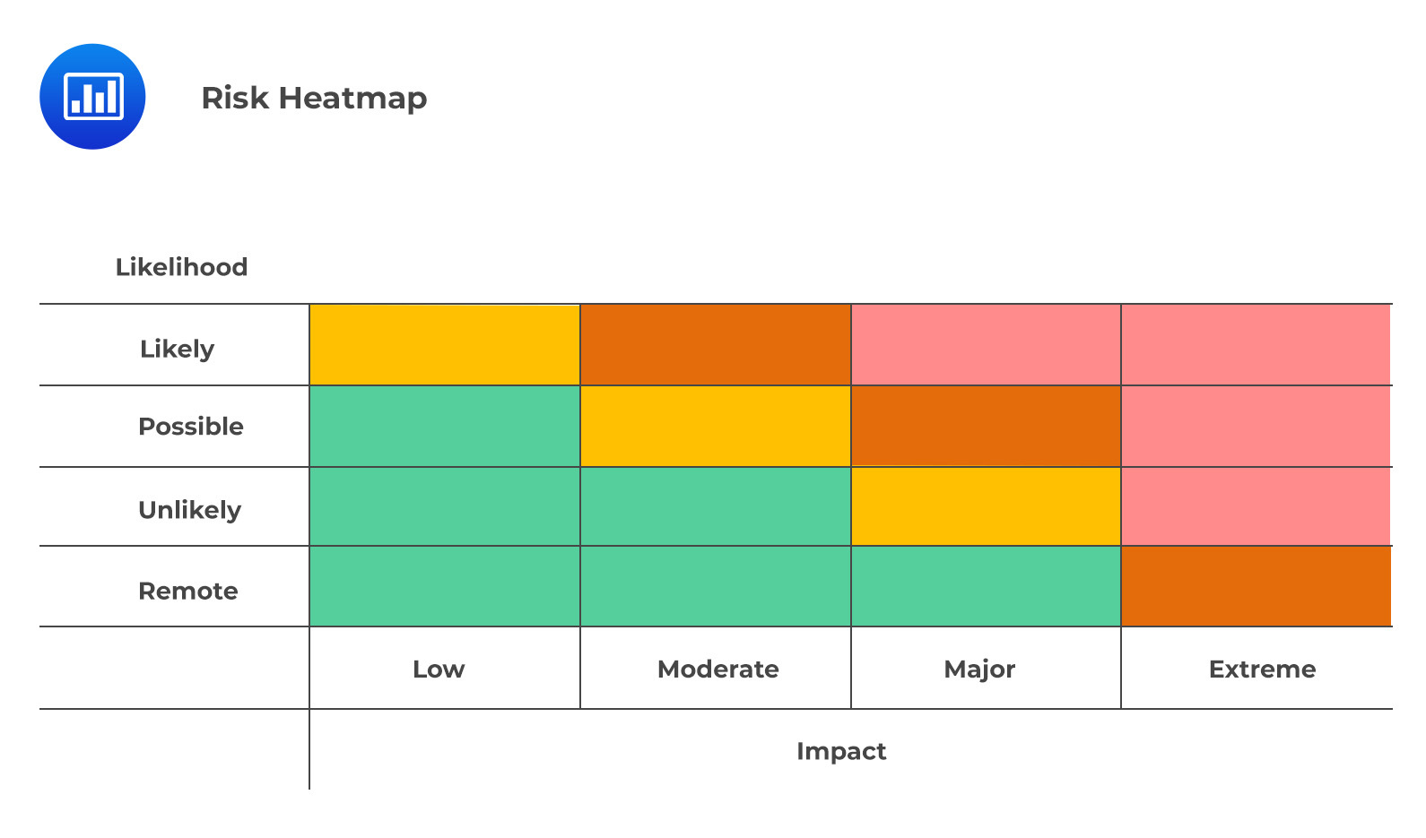It’s important to note that the colors are used in a nonlinear, non-continuous manner. Therefore, it would be a mistake to multiply likelihood and impact to reduce risks to a single numerical quantity. For example, an event that is frequent but low impact (1×4) cannot be the same as an event with a remote probability but an extreme impact (4×1). Therefore, caution should be taken both when manipulating and interpreting the qualitative ratings at play.

The Differences among Key Indicators

Key Risk Indicators (KRIs)

A key risk indicator (KRI) is a metric used in operational risk management to measure an organization’s exposure to potential risks. KRIs provide insight into the likelihood and impact of different types of risk as they evolve over time. Two main types of KRIs exist: preventive KRIs and reactive KRIs.

Preventive KRIs are used to measure the increase or decrease in the likelihood or impact of a potential risk event over time. For example, if a KRI of likelihood shows an increase in the probability that a risk might materialize, then an organization must take preventive measures to mitigate this risk. On the other hand, a KRI of impact, demonstrates how severe a potential risk event could be if it were to occur, allowing organizations to better understand what kind of mitigation strategies should be employed in order to reduce its effects.

Reactive KRIs are used after an incident has already occurred, since they provide key information about actual and potential losses associated with the incident as well as possible root causes and corrective actions taken afterward. This allows organizations to have a clear picture of what went wrong and how it can be prevented from happening again in the future. Additionally, these types of metrics can help organizations identify areas that need improvement when it comes to operational processes and procedures related to certain risks.

Key risk indicators used to measure likelihood include:

• The number of transactions per staff member (could indicate the risk of making errors).
• A drop in customer satisfaction scores (indicating customer attrition).
• An increase in the level of sales required for sales staff to achieve a performance goal.

Key risk indicators used to measure impact include:

• An increase in the amount of responsibility held by key employees (could indicate the impact of discontinuity if the employee leaves the company or is taken ill).
• Increase in sensitivity of data held on a given server (higher impact in case of data leakage/loss).
• Increase in value generated by top-10 clients (higher impact in case of client attrition).

Key Performance Indicators (KPIs)

KPIs measure a company’s performance against predetermined targets. They can be used to evaluate how well a company executes its strategy by comparing the current performance against targets or goals set out in the business plan. KPIs are usually expressed in terms of financial measurements such as revenue growth or return on investment, but in the context of operational risk, they may include:

• Customer service levels.
• Employee engagement scores.
• Maximum downtime.
• Error rates on retail transactions.

By using KPIs, organizations can track progress toward their goals and ensure they take effective action to improve performance if required.

Key Control Indicators (KCIs)

KCIs measure the effectiveness of internal controls within an organization in order to detect fraud or other irregularities. They provide insight into how well existing processes function and alert managers when something appears off—allowing them to take corrective action quickly before any major issues arise. KCIs help to ensure that organizational policies are being observed and that any potential weak spots are identified early on so that appropriate measures can be taken to address them.

Examples of KCIs include:

• Missed due diligence items.
• Lack of segregation of duties.
• Overlooked errors in four-eye checks (reviews by two competent Individuals).
• Incomplete identification files.

It is common for metrics to overlap in their use as performance indicators, risk indicators, and control indicators. Quite often, the same metric can be used for two categories or even all three. The most simplistic example is when actual performance falls below a pre-defined minimum standard. Not only does this indicate weak performance, but it also signals a potential source of risk. An issue with performance can quickly become an issue with risk management if not addressed appropriately. Moreover, delayed financial confirmations of financial transactions can reflect poorly on an organization’s back office efficiency (KPI), create higher possibilities for legal action or fraud (KRI), and point to an organizational failure in applying controls during transaction processing. Understanding these overlapping implications becomes essential to safeguard any operations.

Quantitative Approaches and Models Used to Analyze Operational Risk

Fault Tree Analysis (FTA)

Fault Tree Analysis (FTA) is a type of analysis used to identify the root causes and potential consequences of operational risks. It is a top-down approach that examines the different ways an event or failure can occur, allowing organizations to visualize the sequence of events that lead to an incident. FTA involves creating a fault tree diagram, which is a graphical representation used to depict all of the possible failures that could contribute to an event. This diagram looks like a tree structure with root causes at the top and branches for each subsequent cause-effect relationship that contributes to the incident.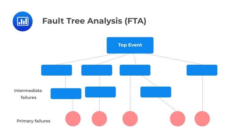

An important part of FTA is performing quantification, which allows for further assessment of operational risks. Quantification involves assigning probabilities to each component of the fault tree in order to create an overall picture of how likely it is for certain events or failures to occur. This helps organizations understand how many components need to be taken into account when implementing preventative measures or contingency plans. Additionally, FTA can help establish which components are most critical in mitigating risks, which will help prioritize efforts during risk management planning.

FTA relies on a series of both dependent and independent conditions that are connected in the form of AND or OR conditions. The joint probability of failure for these conditions can be calculated by multiplying the individual probabilities. For example, if three key independent controls each fail with a 10% likelihood, then their joint probability of failure is \(0.1^3 = \frac{1}{1000}\).

By layering multiple independent controls onto the same system, organizations can reduce the overall risk they face by decreasing the chance that all controls will fail simultaneously. However, even with many layers of safety measures in place, some events may still occur simultaneously due to various external factors or chance occurrences. FTA helps organizations determine what these risks are before they occur and prepare for any necessary contingencies. To achieve this end, FTA provides organizations with a comprehensive view of how their systems interact and what risks they face from all possible combinations of events that could happen at any given moment.

FTA can also be used proactively in order to assess potential risks before they actually occur. By simulating scenarios, organizations can identify new areas where they need additional safeguards and control measures in place in order to minimize operational risk exposure and improve their resilience against future incidents or disruptions. Additionally, FTA can also provide insight into developing trends within operational processes so that organizations can take proactive actions before any issues occur and ensure sustainable business continuity going forward.

Example: Fault Tree Analysis

Let’s consider the following conditions that all need to be present for the scenario to materialize:

1. A malicious external actor targets a company with a phishing email laden with malware. P1.
2. The company’s firewalls fail to detect malicious emails. The firewalls have been misconfigured and lack anti-virus protection. P2.
3. An employee opens the email, unaware of its true intent. P3.
4. The detective controls of suspicious network activity fail. P4.
5. Large amounts of valuable information are stolen from the firm’s systems. P5.

If we assume that these conditions are fully independent, the likelihood of this risk materializing is the simple product of the individual probabilities: P1 × P2 × P3 × P4 × P5. This constitutes the minimum theoretical likelihood of the scenario. For example, if the probability of each of these events is 20%, then the likelihood of this scenario is \(0.20^5=0.00032\).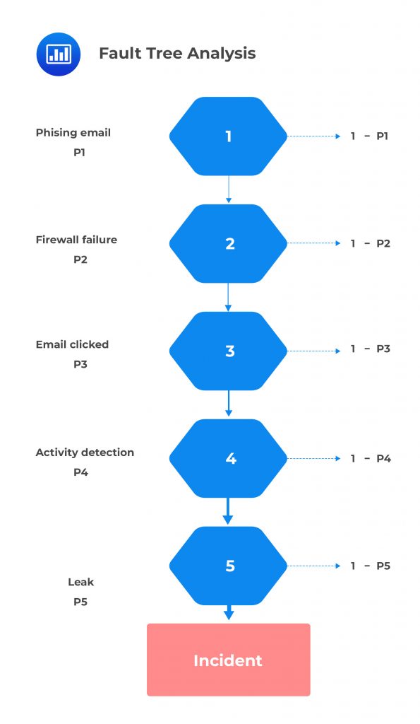

The FAIR Model

The FAIR model is a powerful factor model many financial institutions use to quantify operational risk. The risk factors and their relationships are first identified before measurements and metrics for each factor are calculated. This information is then combined in order to bring about the overall risk value for the organization. What makes the model particularly advantageous is its ability to provide precise analytical processes that give clarity into the various risks, thereby enabling financial institutions to make well-informed decisions when managing operations.

In FAIR methodology, each scenario is composed of:

• An asset at risk: The target that the threat is focused on.
• A threat community: The originator of the threat or its source.
• A threat type: The nature of the threat; whether physical, cyber, or otherwise.
• An effect: The losses caused by the risk manifesting itself.

Business experts must then provide estimates for how frequent losses from these scenarios are likely to occur as well as their magnitude. These estimates should take into account factors such as the likelihood of attack success and expected damage levels.

To further refine outcomes, Monte Carlo simulations are run based on these inputs, which provide a range of potential losses for each scenario. By understanding which assets may be impacted to what extent and probability, organizations can work to bring about measures to safeguard their interests in a cost-efficient manner.

The Swiss Cheese Model

The Swiss Cheese Model is a popular tool for analyzing organizational defenses against failure in health care, aviation, and other highly regulated industries. It suggests that since complex systems cannot be safeguarded completely, it is instead important to ensure that the defenses are built up one layer at a time to fill any gaps and prevent catastrophic situations.

The model was developed by James Reason, a British psychologist, and works by visualizing these multiple levels of defense as holes in slices of Swiss cheese. By picturing the system as a series of slices of Swiss cheese laid side by side, the idea behind this model is that operational risks can arise when the holes in one layer align with those in another, creating a clear path for hazards. Each layer stands for a different barrier or defensive strategy and, when implemented correctly, creates an all-encompassing net against unfavorable outcomes. The idea is that when all the slices are aligned correctly, they can cover any gaps caused by their individual weaknesses resulting in an overall strong defense system.

Owing to its main role in contributing to safety practices globally, the Swiss Cheese Model unarguably features as the most significant development in risk management theory all over the world today.

Root Cause Analysis (RCA)

Root-cause analysis is an important tool for operational risk managers as it allows them to identify the causes of operational issues and implement measures that reduce future risks. RCA is a systematic approach to investigating incidents or near misses by analyzing their root causes, which is defined as the most fundamental factor that led to the occurrence of the incident. By using this approach, the organization can improve its control processes and respond correctly in similar situations in the future.

In banking, root-cause analysis can be used to investigate various events. For example, if a customer experiences fraud or theft from their bank account due to inadequate security measures, RCA can help determine why these security measures were inadequate. The investigation would include looking at whether there were changes in policy or procedure that caused gaps in security; examining technology systems and hardware components to see if they are up-to-date with current standards; evaluating employee training programs to verify they are adequate; and assessing whether any other external factors such as cybersecurity threats could have contributed to the issue.

Once potential causes have been identified through RCA, corrective action plans can be developed in order to reduce future risks. For example, if it was determined that inadequate training was responsible for weak security protocols leading to customer fraud, then steps could be taken to improve employee training programs so that staff members understand best practices when it comes to protecting customers’ financial information. Additionally, policies and procedures could be updated or new ones implemented so that employees are aware of how best to respond when there is an incident relating to sensitive customer data or funds. Banks may also need to invest in more advanced technologies, such as multi-factor authentication, for improved security of their systems and customers’ accounts.

The Bowtie Tool

The Bowtie Tool is a visual application of RCA that can help organizations better understand the interactions between causes and consequences of risk events.

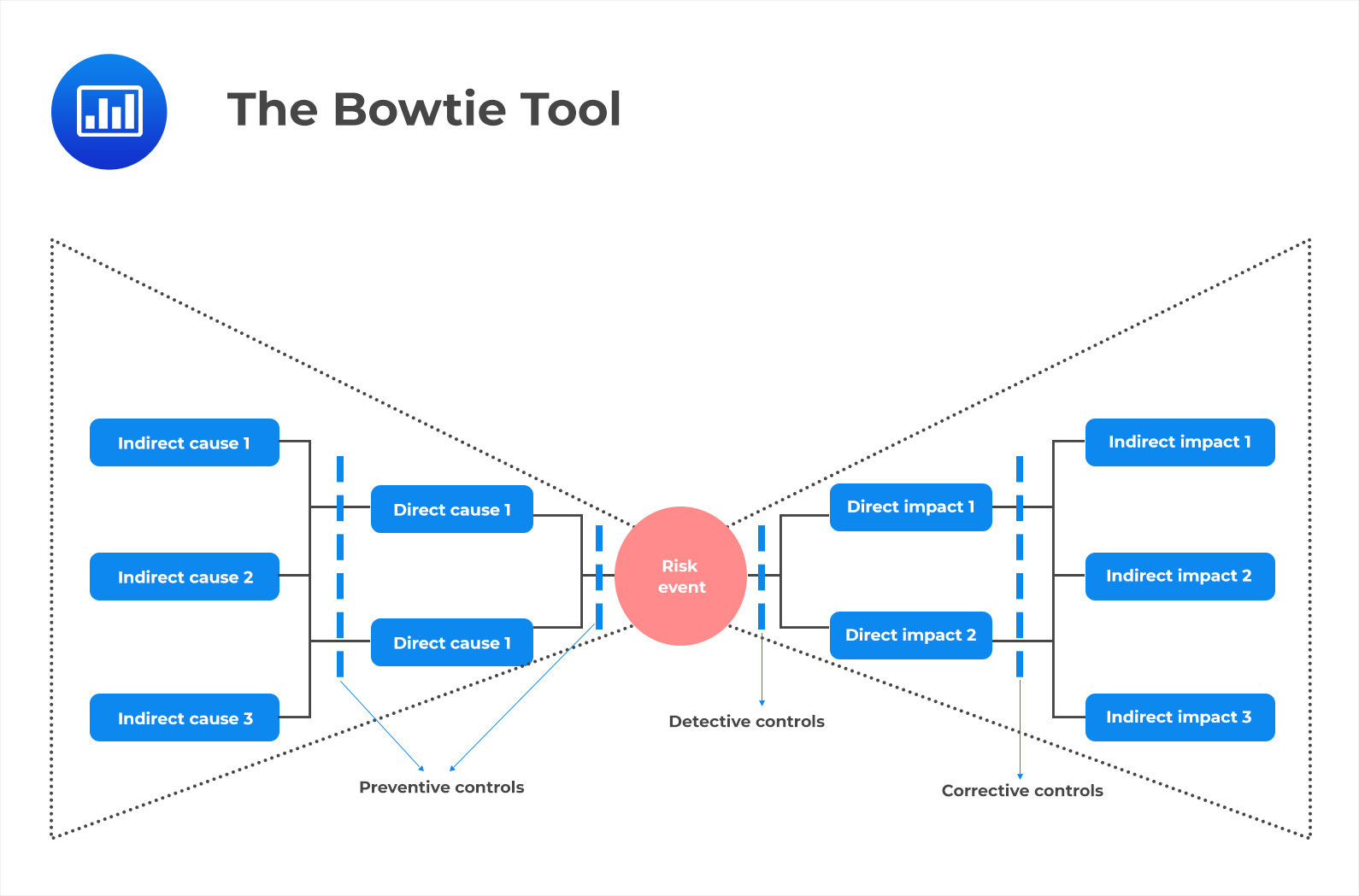
On the left side of the bowtie are direct and indirect causes, as well as preventive controls. Direct causes are the factors that directly lead to an incident, while indirect causes represent preconditions for an incident. These preconditions may include a lack of adequate training, knowledge or skills, technology deficiencies, lack of collaboration or communication among stakeholders, etc.

In the middle is where the actual risk event is identified. This could be anything from a system error or malfunction to an employee making an incorrect decision, or bad judgment call.

On the right side of the bowtie are impacts – the consequences of the risk event. Impacts can range from minor inconveniences all the way up to total catastrophic failure. Also present on the left are detective controls and corrective controls. Detective controls allow organizations to discover any problems quickly so they can take action before too much damage has been done. On the other hand, corrective controls help organizations respond effectively when something goes wrong.

Approaches Used to Determine the Level of Operational Risk Capital for Economic Capital Purposes

Loss Distribution Approach (LDA)

The Loss Distribution Approach (LDA) is an actuarial technique that has been around for some time. It is used to divide loss data into two components: frequency and severity. Frequency refers to the number of times a loss event occurs, while severity measures how costly it is when it does happen. By decompounding each loss event into its constituent frequency and severity components, the amount of available observation data points for modeling activities is doubled.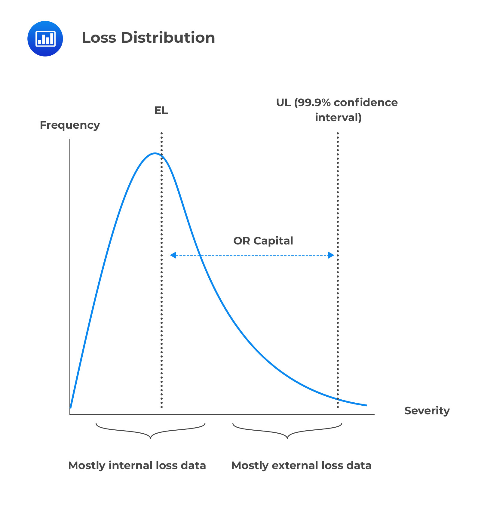

This was especially beneficial in operational risk modeling since there was a severe lack of modeling data at the beginning stages of this field. Two risk modelers from the French bank Credit Lyonnais, Frachot and Roncalli, wrote a groundbreaking paper on applying LDA to operational risk, which has become commonplace ever since. This method has been more popular in continental Europe compared to stress testing and scenario-based modeling, which have been more commonly employed elsewhere.

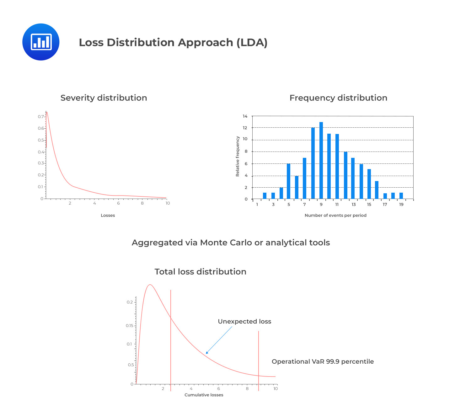
In LDA, frequency and severity distributions are estimated independently, then convoluted into an aggregated loss distribution.

Frequency Modeling

The Poisson distribution is among the simplest frequency distributions as it requires only one parameter for analysis. The parameter lambda (λ) can be used to measure both the mean and variance in the data. When utilized correctly, this model allows for greater insight into an organization’s operational risks and potential events that can occur within any given year or other chosen time frame.

According to Basel II’s 2009 study, 90% of firms use a Poisson distribution when modeling frequency in operational risk, while 10% use negative binomial distributions.

Severity Modeling

Severity is typically modeled using continuous, asymmetric, and heavy-tailed distributions. This is to capture the large number of small events that make up the bulk of operational risk losses, along with a few very large ones. One popular model used to represent severity is the lognormal distribution, which is a logarithmic transformation of the normal (Gaussian) distribution. Moreover, Weibull and Generalized Pareto Distributions (GPD) have been increasingly employed in recent years due to their more heavy-tailed nature. To elaborate further on this, lognormal distributions can be used to approximate data when there is underlying variability between different items or events within a dataset. In contrast, Weibull and GPD are well suited for modeling data points that follow an exponential decay pattern, making them especially useful for predicting future loss events with greater accuracy than traditional methods.

Limitations and Constraints of LDA

LDA assumes independence between the claim frequency and severity, an assumption that’s considered too strong given the stark contrast seen in practice between the frequency of small compared to large operational risk events.

In addition, the assumption of independence and identical distribution (i.i.d.) within each risk class is an oversimplification in many cases; operational risk events can be highly heterogeneous, with significant correlations between loss amounts and various factors such as country, industry segmentation, legal entity, business unit, or other metrics. Additionally, the use of a single data-generating mechanism to generate all losses may not accurately represent the complexity of operational risk events.

Extreme Value Theory

Extreme Value Theory (EVT) is a statistical method of analyzing extreme events in data sets. It can be used to model operational risk capital by examining the distribution of large values, or “outliers”, within a data set. This method of risk capital modeling is based on two main components: Block Maxima (Fisher-Tippet), following the Generalized Extreme Value (GEV) distribution, and Peaks-over-threshold (POT).

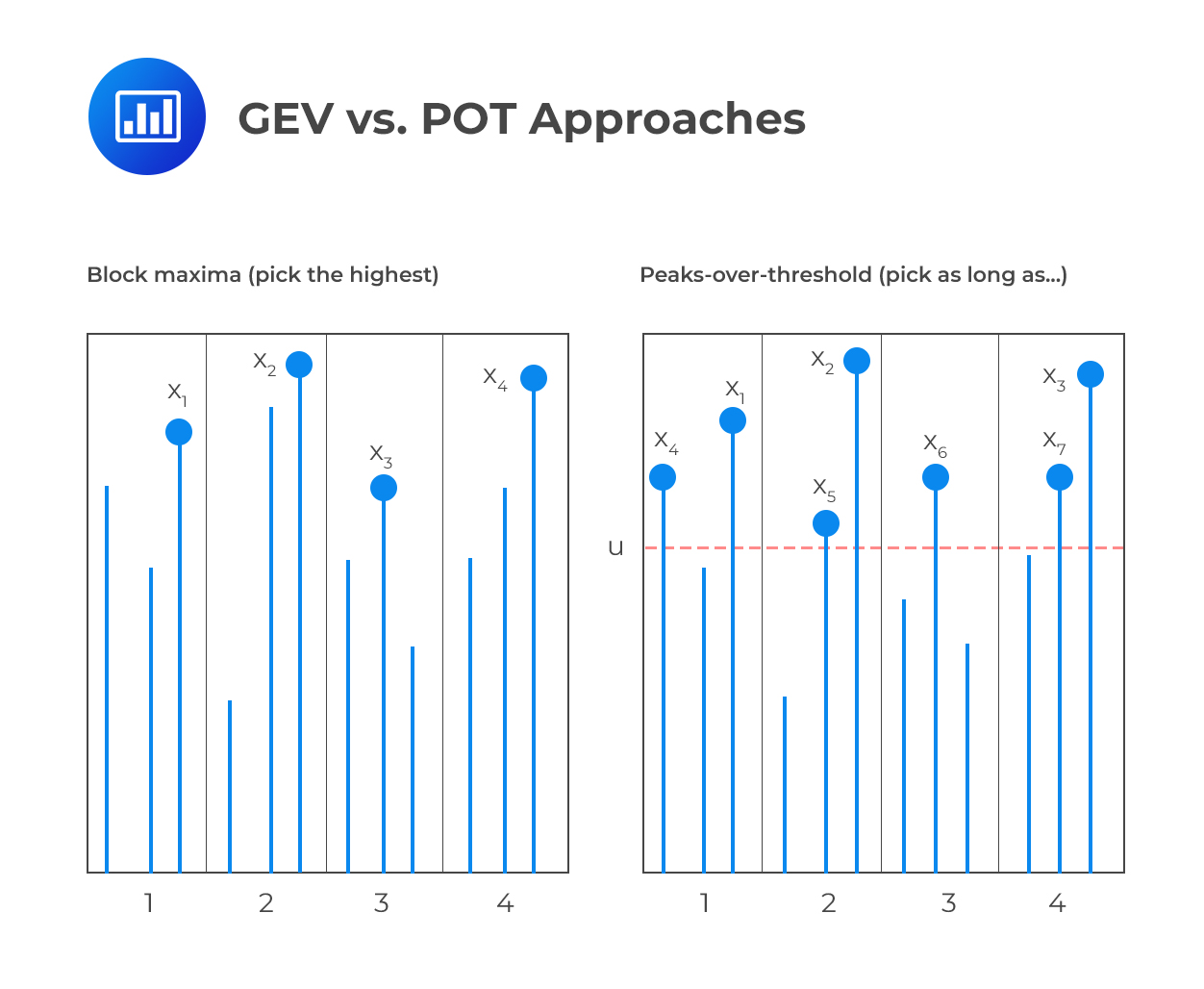
Block Maxima examines the behavior of maxima values which are equally spaced in time (e.g., maximum operational loss per period of time and per unit of measure). This allows for the identification and analysis of maxima patterns that occur over time and their severity level for determining potential risk levels. In addition, this approach takes into account that some observations may not follow the same pattern as others and thus can be omitted from the analysis if deemed necessary.

The second component – Peak-over-threshold – works by focusing on observations that lie above a certain high threshold, “\(u\)”, which is set to be sufficiently large. According to theorem 7, when the threshold is high enough, the excess distribution \(Fu(y)\) converges to the Generalized Pareto Distribution (GPD), providing an approximation of the excess under EVT assumptions.

Limitations of EVT

EVT is only applicable if a single mechanism is responsible for all the observed losses, and this mechanism can be assumed to produce any future losses that exceed the current levels seen in the data. This means that EVT cannot account for fluctuations in different institutions, business lines, or risk types, as each of these has a unique set of variables and drivers of risk.

In addition, EVT generally relies on large amounts of data in order to estimate reliable quantiles with enough accuracy and provide meaningful results. If too little data is available, inaccurate estimates may result, leading to unreliable predictions about future risk levels.

Steps a Firm can Take to Ensure Strong Operational Resilience

Given the potential for operational risk disasters to have a devastating effect on a firm’s revenue and long-term earnings, as well as its reputation and impact on key stakeholders, it is essential that organizations take proactive measures to ensure they are adequately prepared and resilient in the face of such disasters. System failures or disruptions, cyberattacks, physical damage, and compliance issues can all lead to operational risks, many of which may have never been encountered by an organization before.

To ensure resilience, firms should take the following steps:

1. Identify Important Business Services

It is essential for a firm to understand the services that are essential to its success and those which require high availability and resilience. A firm can do this by mapping out the entire service architecture, including all dependencies between systems, applications, and services. The goal should be to gain an understanding of how each component contributes to overall operations and to identify any single points of failure that could lead to critical incidents.

2. Set Impact Tolerances for Important Business Services

Once important business services have been identified, impact tolerances can be set based on the required performance or availability levels for each one. These should reflect the maximum downtime or disruption allowed without causing a significant negative consequence for the organization in terms of reputation, customer satisfaction, or financial loss.

3. Map Important Business Services End-to-End and Identify Resources Required to Deliver Them

A detailed end-to-end map of all important business services should be created showing how each of their components interacts. This will help to identify any needed resources to ensure successful delivery, such as personnel, hardware, software, data sources, etc. 

4. Design Severe but Plausible Scenarios to Test Vulnerabilities in the Delivery of the Important Business Service

Using the impact tolerances set in step two as a guide, severe but plausible scenarios should be developed that test the vulnerability of each service when subjected to extreme conditions such as large-scale cyber attacks or natural disasters. This will provide an indication of any areas where immediate action may need to be taken in order to prevent a major incident from occurring in future operations.

5. Where Impact Tolerance Is Exceeded, Examine Lessons Learned from Stress Tests and Take Actions

If any stress tests exceed the pre-defined impact tolerance then it is important that lessons are learned from them and actions taken accordingly in order to improve operational resilience going forward. For instance, if an incident was caused by a particular resource, such as hardware or software, then steps can be taken to replace it with a more resilient alternative. Alternatively, the attendant risk can be mitigated, if possible, through better configuration or protection mechanisms.

6. Ensure Internal and External Communication Plans are in Place to Be Followed When an Event Occurs

It is also important that communication plans are in place internally between employees and departments that might need to coordinate responses during an incident and externally with customers, suppliers, partners, regulators, etc. who might need notification of what has happened. Having these plans already drawn up allows both sides more time during critical moments instead of having to create them on the fly which could lead to delays in responding appropriately.

7. Annual Self-Assessment Document to Be Signed off by the Board

Finally, it is advisable for firms to conduct regular self-assessments with regard to operational resilience. This document should include recommendations from previous testing sessions along with proposed solutions that could address potential vulnerabilities identified therein. It should also track progress over time, so senior management can closely monitor any trends toward improving operational resilience before being signed off by Board.

How to Test the Operational Resilience of Important Business Services

Scenario analysis is used to model potential operational risk disasters in order to provide expected outcomes that serve both as an input for tail risk distributions and a benchmark for judging the sufficiency of capital allocation.

Scenario analysis helps organizations gain a better understanding of how these risks could potentially materialize and analyze their own resilience if such situations do arise. While not every disaster can be predicted or anticipated ahead of time, scenario analysis allows organizations to at least attempt to anticipate various risks they could face while also attempting to come up with strategies to mitigate them should they occur. By having these plans in place ahead of time organizations can be better prepared when they do encounter operational risk disasters.

In addition, regulations requiring organizations to consider such plausible disasters also require that firms assess their resilience plans regularly. This is done so that firms can continue improving their ability to withstand any future catastrophes that may arise from system failures or disruptions, cyberattacks, physical damage, or compliance breaches. This requires firms to take into account not just what has happened in the past but also potential future events as well in order for them to stay ahead of the curve when it comes to managing potential operational risks.

Practice Question 

Joel and Mark, FRM Part II candidates, are discussing BCBS’ guidelines on the need to report comprehensive data regarding operational risk events. During the discussion, the following statements are made.

Which statement is most likely correct?

1. While the Basel Committee has set a minimum threshold for loss reporting at €20,000 ($22,000), setting reporting thresholds at zero is considered the best practice so as to capture every operational loss or simplify instructions to the business units that do not need to estimate a loss before deciding to report incidents.
2. Regulatory guidelines dictate that firms must report any incidents causing them both financial losses and non-financial impacts.
3. Both direct and indirect losses must be reported.
4. Grouped losses are distinct operational risk events connected through a common loss amount.

The correct answer is C.

It is important to remember that both direct and indirect losses must be reported. Direct losses are the ones incurred immediately after an event. Examples of such losses include: the cost of remediation, any financial outcomes due to wrongful transactions, or compensation to clients. Indirect losses are much trickier to identify since they are results of further consequences from an operational risk event.

A is incorrect. Even though some banks do set a threshold of zero for operational risk events, this strategy is fading away among large banking institutions. This trend is attributed to the sheer number of small incidents that must be reported with little information value gained in return. Instead, most banks and insurance companies prefer a threshold slightly lower than the regulatory limit. Thresholds of €20,000, €10,000, or €5,000 are common.

B is incorrect. Banks are only required to report any incidents causing them financial losses. But from a management perspective, it’s also good practice to record the non-financial impacts associated with any material operational risk events.

D is incorrect. Grouped losses are defined as distinct operational risks connected to a single core event or cause. For example, if an IT failure occurs, impacting various departments in different ways, this sequence of events would likely constitute one grouped loss.

Things to Remember

• BCBS guidelines provide a framework to ensure uniformity and comprehensiveness in reporting operational risk events across financial institutions.
• While thresholds for loss reporting can vary, the key is ensuring significant operational risks are captured and not overlooked.
• Operational risk reporting isn’t solely about financial quantification; understanding the nature, cause, and context of the risk is equally critical.
• Regular and meticulous reporting aids in refining risk management strategies and enhancing operational resilience.
• Adhering to these guidelines not only ensures regulatory compliance but also fosters trust among stakeholders and clients.