Validating Bank Holding Companies’ V ...
After completing this reading, you should be able to: Describe some important considerations... Read More
After completing this reading, you should be able to:
A binomial model is a model that assumes that interest rates can take only one of two possible values in the next period. It is depicted in form of a tree that has a set of nodes with discrete spacing and times. A node is a point in time when interest rates can take one of two possible paths. At time 0, there is one root node with the current interest rate. From there it leads to two other nodes which show the alternative interest rates in the next period. As time goes by, more and more possibilities emerge, resulting in some kind of a complex network that can extend to several periods into the future.
As noted earlier, a node is a point in time when interest rates can take one of two possible paths – an upper path, U, or a lower path L. Each node to the right of the tree results when the initial rate \(\text i_0\) follows a specific path. For example, to arrive at the top-most node, \(\text i_{2,\text{UU}}\), the initial rate follows the upper path from node 0 to node 1 to become \(\text i_{1,\text U}\). From here, it takes the upper of the two possible paths to node 2. Similarly, to arrive at the lowermost node, \(\text i_{2,\text{LL}}\), the initial rate follows the lower path from node 0 to node 1 to become \(\text i_{1,\text L}\). It then takes the lower of the two possible paths to node 2. From node 0, an upward move followed by a downward move or a downward move followed by an upward move gets us to the same point, \(\text i_{2,\text{LU}}\).
The interest rates at each node are 1-period forward rates corresponding to the nodal period. These rates are functions of the volatility assumption used to generate the binomial tree.
To find the value of the bond at a particular node, we use the backward induction valuation methodology. Bonds are redeemed at par. Therefore, we start at maturity, fill in those values, and work back from right to left to find the bond’s value at the desired node. In other words, given a bond that has N compounding periods, the bond’s current value is determined by computing its possible values at period N and working “backward” to node 0.
For a zero-coupon bond, the only cash flow occurs at maturity. To find the value of a bond at a given node in a binomial, tree we find the average of the present values of the two possible values from the next period. The appropriate discount rate is the forward rate associated with the node under analysis.
One of the most important rules underlying the construction of binomial trees is that there should be no arbitrage, i.e., the values for on-the-run issues generated using an interest rate tree should prohibit arbitrage opportunities. The value of the issue produced by the binomial tree must equal the market price.
The figure below shows a binomial tree of a $1,000 face value zero-coupon bond with two years remaining to maturity. The block at the first node and the other pair of blocks at end of year 1 include the value of the bond and the 1-year forward rate. The blocks on the far right give the bond’s par value. Assuming that the bond’s market price is $900 and that up and down moves have equal probability, we can demonstrate that the tree in figure 1 is arbitrage-free using the concept of backward induction. So, how do we go about it?
We work from right to left:
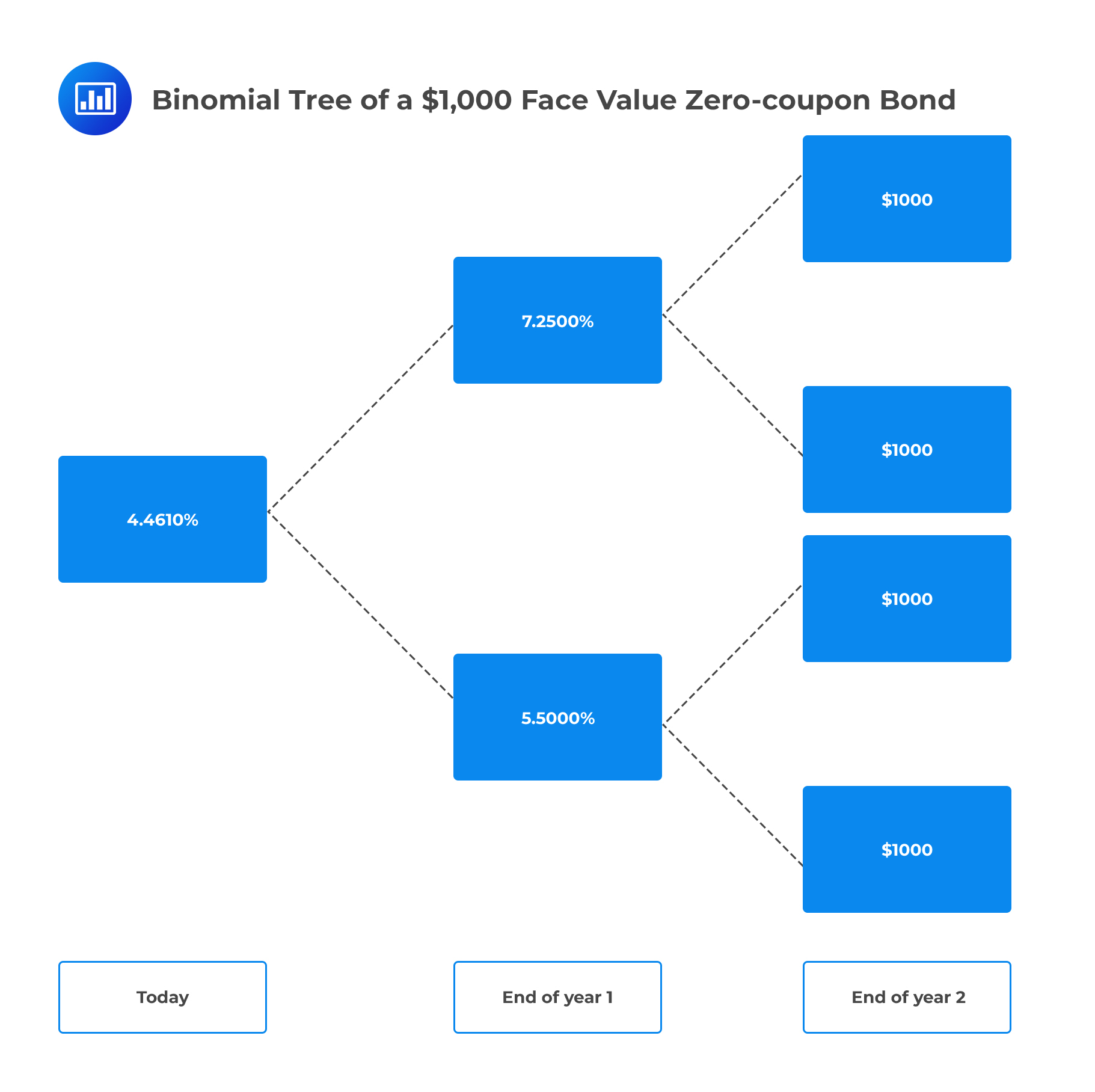 Consider the value of the bond at the upper node for period 1, \(\text V_{1,\text U}\):
$$ \text V_{1,\text U}=\cfrac {$1,000×0.5+$1,000×0.5}{1.0725}=$932.40 $$
Similarly, the value of the bond at the lower node for period 1, \(\text V_{1,\text L}\):
$$ \text V_{1,\text L}=\cfrac {$1,000×0.5+$1,000×0.5}{1.055}=$947.87 $$
From this point, we calculate the current value of the bond at node \(0, \text V_0\):
$$ \text V_0=\cfrac {$932.40×0.5+$947.87×0.5}{1.04461}=$900 $$
Since the computed value of the bond equals the market price, the binomial tree is arbitrage free.
For the calculations above, we assumed that interest rates are compounded annually. Similar calculations can be done when the interest rates are compounded semiannually.
The no-arbitrage pricing approach for valuing a derivative consists of three main steps:
Consider a call option on a $1000 par of a zero maturing at time 1. The call gives the owner the right but not the obligation to buy the underlying bond for the strike price at the expiration date. Further, suppose that the expiration date is time 0.5, and the strike price $975.
Working assumptions:
Determine the price of the call.
Step 1: Describing the future payoff or price of the underlying assets across different possible states
If the six-month rate on date 1 turns out to be 6.0% (the upstate), the price of the then six-month zero will be $970.87
$$ \cfrac {1,000}{\left(1+\frac {0.06}{2}\right)^1} =970.87 $$
In this case, the right to buy zero at $975 will be worth zero (There’s no point exercising the option).
If the six-month rate on date 1 turns out to be 4.0% (downstate), the price of the six-month zero will be $980.40
$$ \cfrac {1,000}{\left(1+\frac {0.04}{2} \right)^1} =980.4 $$
In this case, the right to buy the zero at $975 (call option strike) will be worth $5.4.
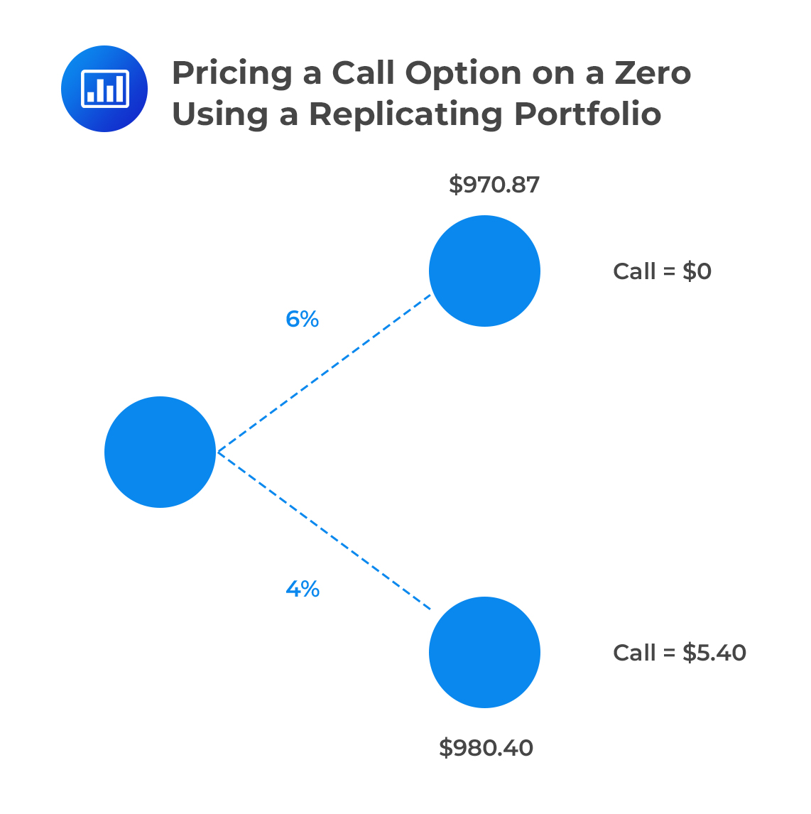 Step 2: Construct a replicating portfolio that has the same random payoff as the derivative.
To price the option by arbitrage, an analyst must construct a replicating portfolio today (date 0) of underlying securities, namely six-month and one-year zero-coupon bonds, that will be worth $0 in the upstate on date 1 and $5.4 in the downstate.
Let the face value of the six-month zero in the replicating portfolio be \(\text F_{0.5}\), and, the face value of the 1-year zero in the replicating portfolio be \(\text F_1\). These values must satisfy the following equations:
$$ \begin{align*} & \text F_{0.5}+\cfrac {1}{\left(1+\frac {0.06}{2} \right)^1} \text F_1 \equiv \text F_0.5+0.9709 \text F_1=0 \\ & \text F_{0.5}+\cfrac {1}{\left(1+\frac {0.04}{2} \right)^1} \text F_1 \equiv \text F_0.5+0.9804 \text F_1=5.4 \\ \end{align*} $$
Solving these equations,
$$ \begin{align*} −0.9709\text F_1 & = 5.4 − 0.9804 \text F_1 \\ \text F_1 & = 568.4 \\ \text F_{0.5} & = 5.4 − 0.9804 × 568.42 = −551.88 \\ \end{align*} $$
Therefore, on date 0, the option can be replicated by buying about $568.42 face value of one-year zeros and simultaneously shorting about $551.88 face amount of six-month zeros.
Step 3: Setting the price of the derivative equal to the value of the replicating portfolio.
By the law of one price,
$$ \begin{align*} \text{Price of call option}& =\text {Price of the replicating portfolio}\\ & =\cfrac {1}{\left( 1+\frac {0.05}{2} \right)^1} \text F_{0.5}+\cfrac {1}{(1+\frac {0.053}{2})^1} \text F_1 \\ & = −538.41 + 539.43 = $15.31\\ \end{align*} $$
Bottom line:
A portfolio of the underlying and riskless asset replicates the call if it satisfies two equations:
Every single event has some probability of occurrence. A good case in point is the probability of the price of a stock either going up or going down. That’s what we call the true probability. Although true probabilities are intuitive, they are not directly useful in finding the price of an option. This is because price is not the weighted average of future outcomes.
In the previous example where we valued an option-free bond, the probability for up and down states was taken to be 0.5. However, these probabilities may not produce an expected discounted value that exactly matches the market price of the bond because they are assumed to be true probabilities.
Risk-neutral probabilities are the probabilities that cause the expected discounted value to equal the market price. They are probabilities of potential future outcomes adjusted for risk.
Any difference between the risk-neutral and true probabilities is referred to as the interest rate drift.
Risk-neutral pricing is a technique that modifies an assumed interest rate process so that any contingent claim can be priced without having to construct and price its replicating portfolio. The idea of risk-neutral pricing is that the binomial option pricing formula can be interpreted as a discounted expected value. The option value at a given node is a discounted expected payoff to the option calculated using risk-neutral probabilities.
To value an option on a fixed-income instrument using a binomial tree, there are three basic steps.
Step 1:Price the bond value at each node using the projected interest rates.
 Step 2:Calculate the intrinsic value of the derivative at each node at maturity.
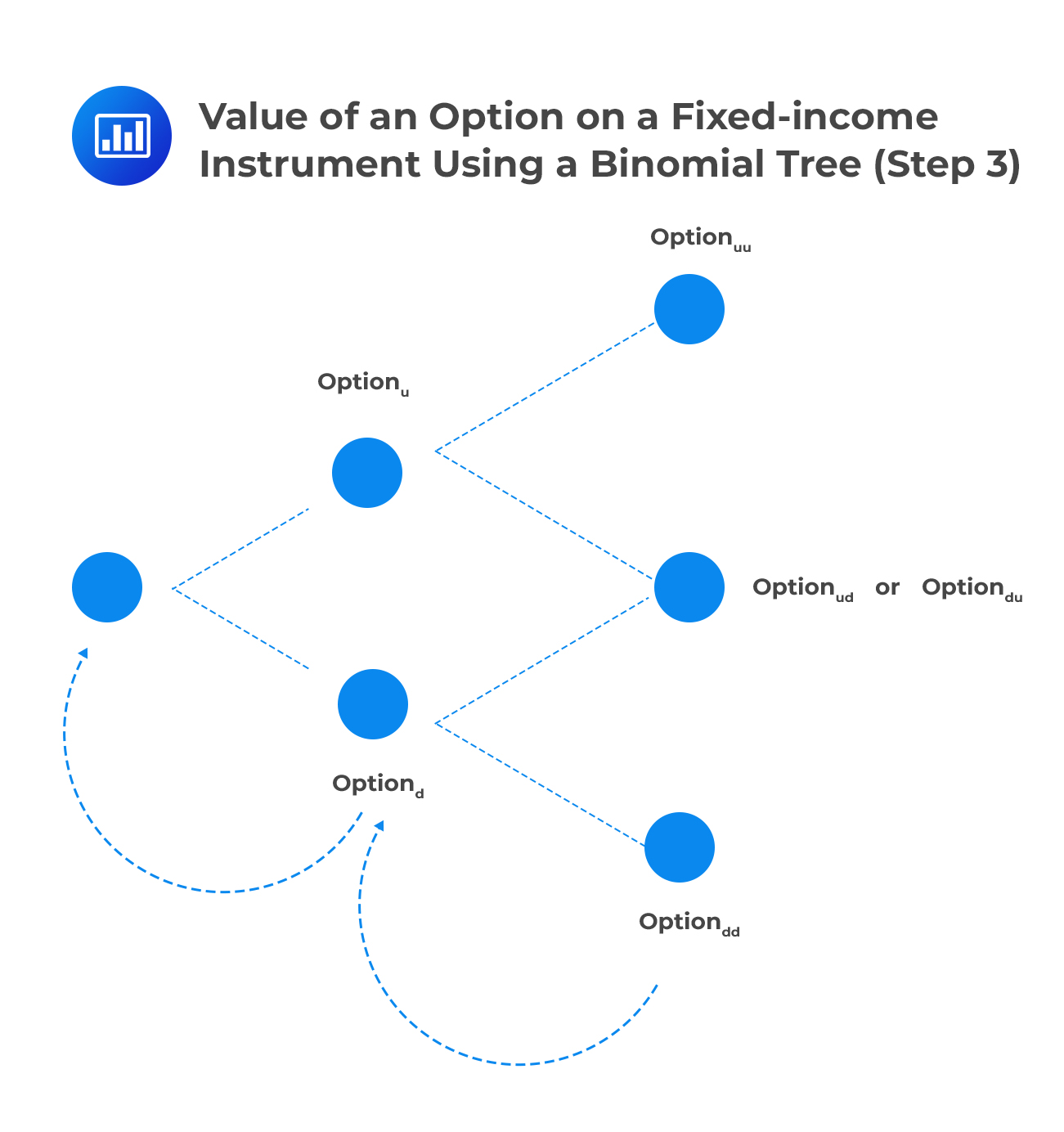
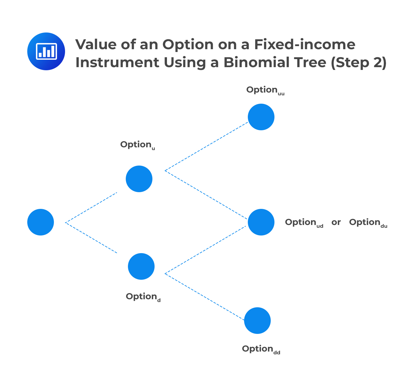 Step 3:Calculate the expected discounted value of the derivative at each node using the risk-neutral probabilities and working backward through the tree.
 Recombining Tree
A recombining tree is a binomial tree that always has just one more ending node in the final period than the number of time steps. For example, in combining a tree that has two-time steps, there will be 3 nodes in the second period.
In contrast, a non-recombining lattice of n time steps has 2n ending nodes. For example, in a non-recombining tree that has two-time steps, there will be 4 nodes in the second period. A non-recombining tree may result when any interest rate above a certain level (say, 5%) causes rates to move a fixed number of basis points. Note, however, that any interest rate below that level causes rates to move at a pace that is below the up state’s fixed amount.
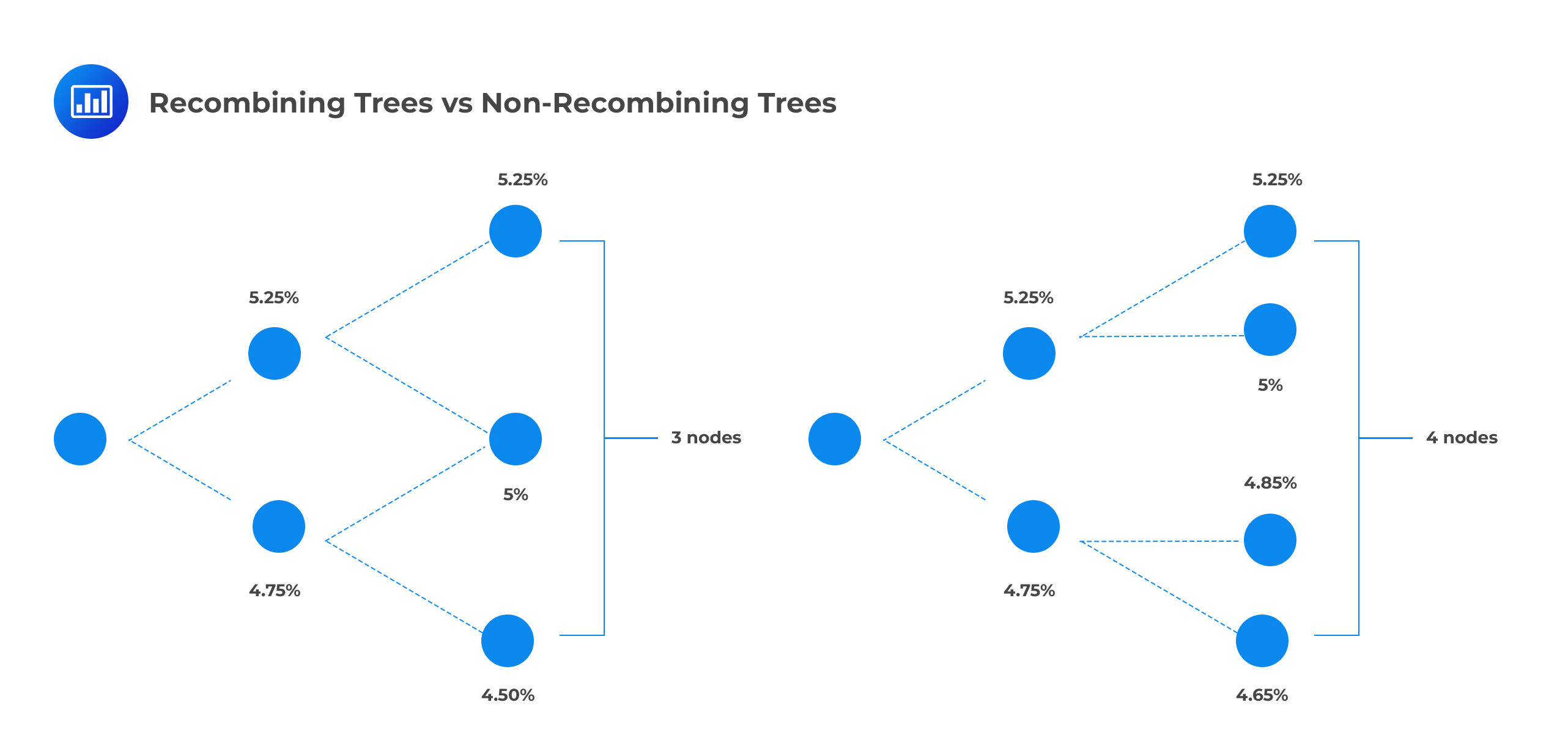 Practitioners “tend to avoid” non-recombining trees because they are difficult or impossible to implement.
A CMT swap is an agreement to swap a floating rate for a Treasury rate such as the 10-year rate. We can use binomial trees to price swaps.
A constant maturity swap pays the following every six months until maturity.
$$ \cfrac {$1,000,000}{2}×\left( \text y_{\text{CMT}}-6\% \right) $$
\(\text y_{\text{CMT}}\)s a semiannually compounded yield, of a predetermined maturity, at the time of payment (\(\text y_{\text{CMT}}\) is equivalent to 6-month spot rates). Further, assume that there is a 70% risk-neutral probability of an increase in the 6-month spot rate and a 60% risk-neutral probability of an increase in the 1-year spot rate.
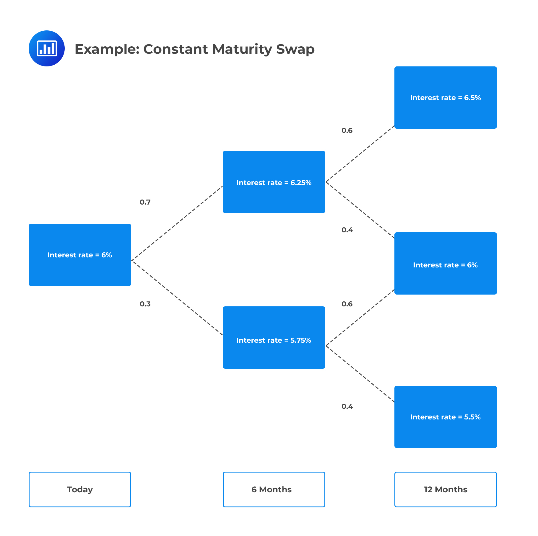 Calculate the value of the swap.
In six months, the top node and bottom node payoffs are, respectively:
$$ \begin{align*} \text{payoff}_{1,\text U} & =\cfrac {$1,000,000}{2} ×(6.25\%-6\%)=$1,250 \\ \text{payoff}_{1,\text L} & =\cfrac {$1,000,000}{2}×(5.75\%-6\%)=-$1,250 \\ \end{align*} $$
Similarly in 12 months, the top, middle, and bottom payoffs are, respectively:
$$ \begin{align*} \text{payoff}_{2,\text U} & =\cfrac {$1,000,000}{2}×(6.5\%-6\%)=$2,500 \\ \text{payoff}_{2,\text M} & =\cfrac {$1,000,000}{2}×(6\%-6\%)=$0 \\ \text{payoff}_{2,\text L} & =\cfrac {$1,000,000}{2}×(5.5\%-6\%)=-$2,500 \\ \end{align*} $$
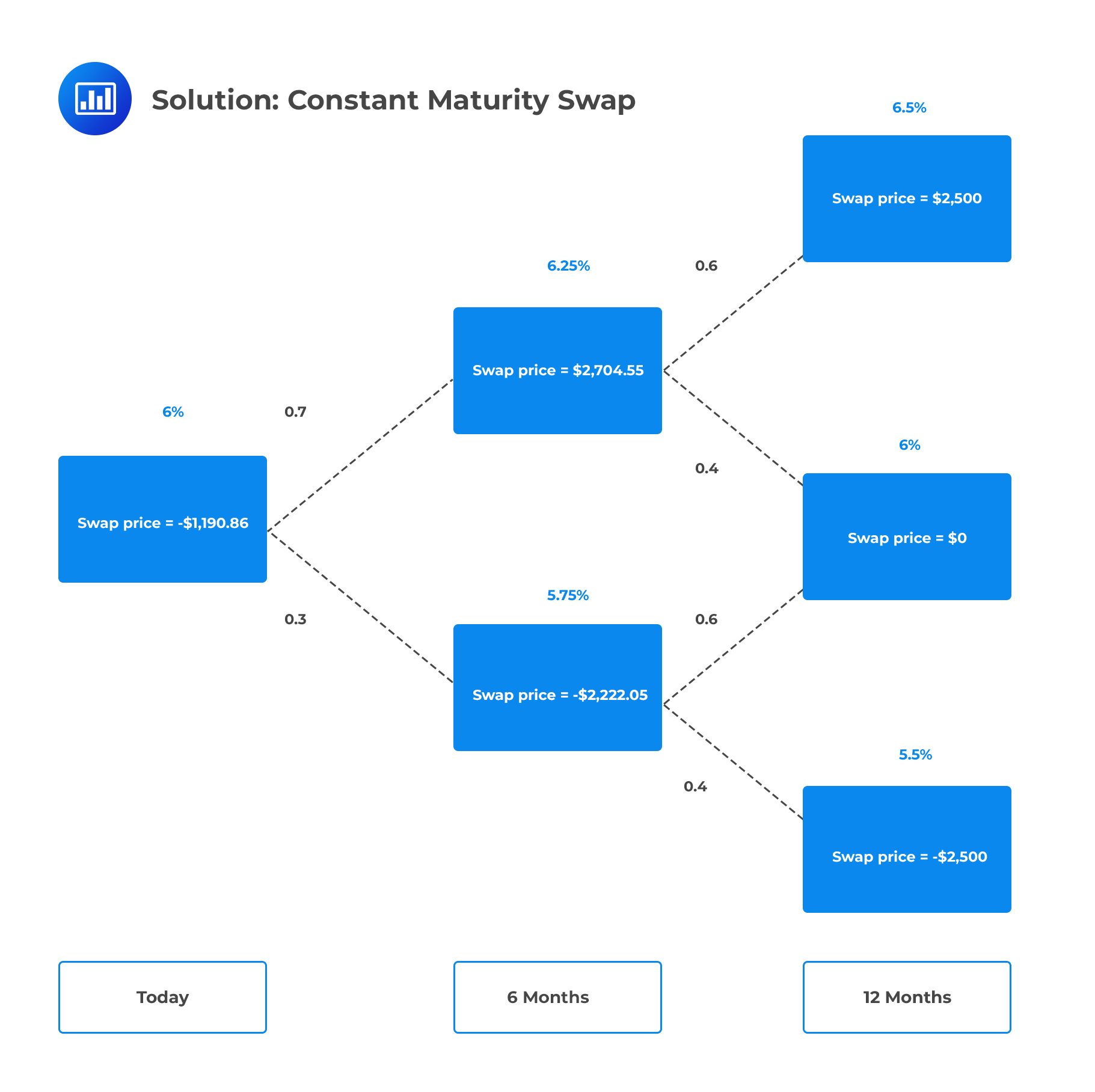
The possible prices in six months are given by the expected discounted value of the 1-year payoffs under the risk-neutral probabilities, plus the 6-month payoffs ($1,250 and -$1,250). Hence, the 6-month values for the top and bottom node are, respectively:
$$ \begin{align*} \text V_{1,\text U} & =\cfrac {($2,500×0.6)+($0×0.4)}{1+\frac {0.0625}{2}+}$1,250 =$2,704.55 \\ \text V_{1,\text L} & =\cfrac { ($0×0.6)+(-$2,500×0.4)}{1+\frac {0.0575}{2}}-$1,250=-$2,222.05 \\ \end{align*} $$
The price today is calculated as follows:
$$ \text V_0=\cfrac { ($2,704.55×0.7)+(-$2,222.05×0.3)}{1+\frac {0.06}{2}}=$1,190.86 $$
 Option-adjusted Spread
The option-adjusted spread (OAS) is the spread that makes the model value (calculated by the present value of projected cash flows) equal to the current market price. In other words, OAS is the spread such that the market price of a security equals its model price when discounted values are computed at risk-neutral rates plus that spread.
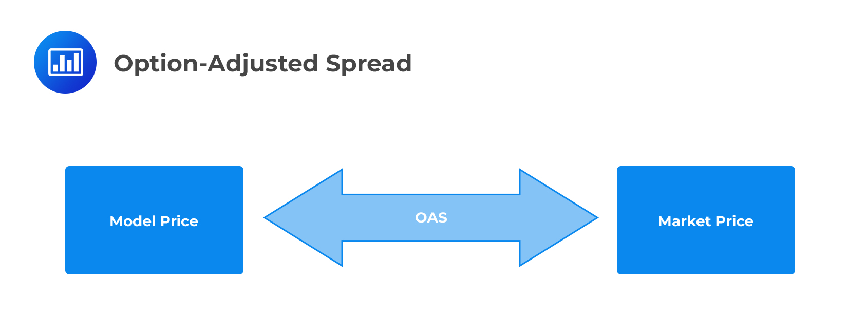 To illustrate this, say that the market price of the CMT swap in the previous section is $1,189.92, $0.94 less than the model price ($1,190.86). In this case, the OAS of the CMT swap turns out to be 10 basis points. To see this, add 10 basis points to the discounting rates of 6.25% and 5.75%.
$$ \begin{align*} \text V_{1,\text U}&=\cfrac {($2,500×0.6)+($0×0.4)}{1+\frac {0.0635}{2}} +$1,250=$2,703.84 \\ \text V_{1,\text L}&=\cfrac {($0×0.6)+(-$2,500×0.4)}{1+\frac {0.0585}{2}}-$1,250=-$2,221.58 \\ \end{align*} $$
Important: Only rates adjusted by the OAS spread are the rates used for discounting values. The OAS does not impact the rates used for estimating cash flows.
To complete the valuation with an OAS of 10 basis points, use the results \(\text V_{1,\text U}\) and \text \(V_{1,\text L}\) and a discount rate of 6% plus the OAS spread of 10 basis points, or 6.10%, to obtain an initial CMT swap value of:
$$ \text V_0=\cfrac {($2,703.84×0.7)+(-$2,221.58×0.3)}{1+\frac {0.061}{2}}=$1,189.92 $$
As illustrated above, discounting at the risk-neutral rates plus an OAS of 10 basis points produces a model price equal to the given market price of $1,189.92.
If a security’s OAS is positive, its market price is less than its model price, so the security trades cheap. If the OAS is negative, the security trades rich.
So far, we have used time steps of w=either 6 months or 1 year. In practice, time steps smaller than six months are desirable for two main reasons:
Smaller time steps, however, have a few disadvantages:
Bottom line: The choice of the number and size of time steps ultimately depends on the problem at hand. Generally, more time steps are preferred for long-term securities such as a 30-year bond, while fewer time steps are preferred for short-term securities such as a one-month bond option.
In a nutshell, the Black-Scholes-Merton model for valuing stock options works under the assumption that the stock price evolves according to a particular random process and that the short-term interest rate is constant. Hence, it is possible to replicate the payoff of an option by forming a portfolio of stocks and short-term bonds. Therefore, by arbitrage arguments, the price of the option must equal the known price of the replicating portfolio.
Unfortunately, the BSM model is hinged on three assumptions that do not apply to fixed-income securities:
Question
A $10 million face value of a stylized constant-maturity treasury (\(CMT\)) swap is struck at 10%. It is a one-year \(CMT\) swap on the six-month yield in 0.5% increments. Calculate the possible values of the \(CMT\) swap after one year.
- $50,000, $0 and -$50,000
- $25,000, $0 and -$25,000
- $100,000, $0 and -$100,000
- None of the above
The correct answer is A.
The \(CMT\) swap pays:
$$ $10,000,000\frac { { y }_{ CMT }-10\% }{ 2 } $$
In 6 months, the state 1 and 0 payoffs are, respectively:
$$ \begin{align*}$10,000,000\frac { 10.5\%-10\% }{ 2 } &=$25,000 \\ $10,000,000\frac { 9.5\%-10\% }{ 2 } &=-$25,000 \end{align*}$$
In 1 year, the state 2, 1 and 0 payoffs are:
$$ \begin{align*}$10,000,000\frac { 11\%-10\% }{ 2 }& =$50,000 \\ $10,000,000\frac { 10\%-10\% }{ 2 }& =0 \\ $10,000,000\frac { 9\%-10\% }{ 2 }& =-$50,000\end{align*} $$