VaR Mapping

After completing this reading, you should be able to:

• Explain the principles underlying VaR mapping, and describe the mapping process.
• Explain how the mapping process captures general and specific risks.
• Differentiate among the three methods of mapping portfolios of fixed income securities.
• Summarize how to map a fixed income portfolio into positions of standard instruments.
• Describe how the mapping of risk factors can support stress testing.
• Explain how VaR can be used as a performance benchmark.
• Describe the method of mapping forwards, forward rate agreements, interest rate swaps, and options.

Principles Underlying VaR Mapping and the Mapping Process

Mapping refers to the process of replacing the current values of a portfolio with risk factor exposures. More generally, it is the process of replacing each instrument by its exposures on selected risk factors. Through mapping, a complex portfolio or instrument can be broken down into its constituent elements that determine its value.

Why is risk mapping necessary? There are four main reasons:

1. Mapping is necessary when we do not have sufficient data on positions.

   In this regard, consider an emerging market instrument that has a very short trading record, meaning that we do not have enough data on it. In such circumstances, we might map our position to some comparable position for which we already have plenty of data and whose risk exposure, we have a good understanding of.

2. Mapping helps us to cut down on the dimensionality of covariance matrices and correlations.

   Given a portfolio comprising of n instruments, we would need to gather data on n volatilities and n(n-1)/2 correlations, resulting in a labyrinth of pieces of information. As n increases, so does the amount of information we have to collect and process. It is important to keep the dimensionality of our covariance matrix at a manageable level to avoid computational problems.

3. Mapping helps avert rank correlation problems.

   By handling a large number of risk factors that are closely correlated (or even perfectly correlated in extreme cases), we might run into rank problems with the covariance matrix and end up producing pathological estimates that might lead to erroneous conclusions. To avoid such problems, it is important that we select an appropriate set of risk factors that are not closely related.

4. Mapping greatly reduces the time needed to carry out a risk assessment and related calculations.

   The reduction of a portfolio comprised of a large number of different positions and a consolidated set of risk-equivalent positions in basic risk factors enhances the capacity to conduct calculations at a faster speed. The only downside to such a move is loss of precision. 

Principles Underlying Mapping

The principles underlying risk mapping can be summarized as follows:

• VaR mapping helps us to aggregate different portfolio positions based on common underlying risk factors. This process becomes particularly useful in cases where evaluating each position separately would be computationally intensive./li>
• Mapping is useful for measuring changes over time. When managing the risk attached to bonds, for instance, risk exposure can be mapped to spot yields that reflect the current position.
• Mapping can be quite useful when historical data is not available.

Mapping Process

Step 1: Mark all positions to market value (in current dollars or reference currency).

This involves the establishment of the current market value of all positions.

Step 2: Identify common risk factors for different investment positions.

A good example of a common risk factor could be a specific exchange rate, say, the Euro versus the dollar.

Step 3: Allocate the market value for each position/instrument to the risk factors.

Figure 1 illustrates this process where 5 instruments are mapped on three risk factors.

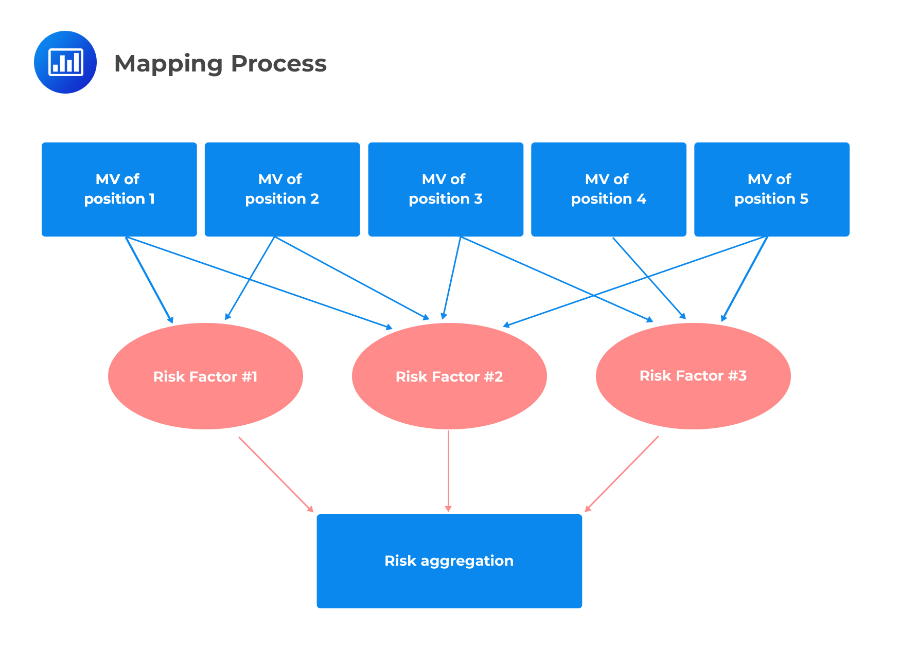Step 4: Construct a risk factor distribution and input all data into the risk model.

The market value of position number 1, for example, is allocated to the risk exposures in the first row, \(x_{1,1} , x_{1,2}, \text{ and } x_{1,3}\).

Step 5: Sum the risk factors in each column then create a vector consisting of three risk exposures.

$$ \begin{array}{c|c|c|c|c} { \textbf{Investment}/ } & {\textbf{Market value}} & {\textbf{Risk Factor 1}} & {\textbf{Risk Factor 2}} & {\textbf{Risk Factor 3}} \\ {\textbf{Position}} & {} & {} & {} & {} \\ \hline {1} & {\text{MV}_1} & {x_{11}} & {x_{12}} & {x_{13}} \\ \hline {2} & {\text{MV}_2} & {x_{21}} & {x_{22}} & {x_{23}} \\ \hline {3} & {\text{MV}_3} & {x_{31}} & {x_{32}} & {x_{33}} \\ \hline {4} & {\text{MV}_4} & {x_{41}} & {x_{42}} & {x_{43}} \\ \hline {5} & {\text{MV}_5} & {x_{51}} & {x_{52}} & {x_{53}} \\ \hline {\text{Total portfolio}} & {\text{MV}} & {x_1=\sum_{i=1}^5 x_{i1}} & {x_2=\sum_{i=1}^5 x_{i2}} & {x_3=\sum_{i=1}^5 x_{i3}} \\ \end{array} $$

The six positions above could be any six instruments, say, forward contracts on the same currency but with different maturities. Through mapping, these positions can be replaced by exposures to three risk factors only – factors 1, 3, and 3.

The idea of risk mapping can be seen in William Sharpe’s diagonal model where he attempts to simplify risk measurement in a portfolio made up of many stock positions. The model decomposes individual stock return movements into two components: a common index component and an idiosyncratic component. The latter disappears as more and more positions are added to the portfolio, leaving the common index component as the main driver of risk.

How the Mapping Process Captures General and Specific Risks

Just how many general (primitive) risk factors do we work with? This is the key question as we engage in any mapping exercise. One or two factors can be convenient to work with, and the process takes less time. Having more risk factors may lead to a better approximation of the portfolio’s risk exposure, but there is a downside. As the number of risk factors increases, the model becomes more complex, and risk modeling takes more time. Therefore, the choice of the set of primitive risk factors should reflect an appropriate tradeoff between a better quality of the approximation and faster processing.

Perhaps, the most important is to recognize that the choice and number of general risk factors will directly affect the size of specific risks. Specific risks are the risks that affect specific assets in the portfolio. They are issuer-specific as opposed to market-related or general risk.

To demonstrate just how the choice and number of general risk factors affect the size of specific risks, consider a portfolio of bonds with different maturities, ratings, terms, and different denominations. Let’s say we start with duration as the only risk factor. In this case, there will be a significant proportion of specific risks. If we add another risk factor, say, for credit risk, we would expect the amount of specific risk to reduce. If we add yet another factor for currency risk, specific risk would shrink even further.

Example:

Let’s assume that we have a portfolio of N stocks and map each stock to the market index, which we define as our primitive risk factor.

The risk exposure, \(\beta_i\), is computed by regressing the return of stock i on the market index return using the following equation:

$$ R_i=\propto_i+\beta_i R_M+\epsilon_i $$

Ignoring the first term,\(\propto\), which does not contribute to risk, the portfolio return, given that the relative weight of each stock is \(w_i\), is:

$$ R_p=\sum_{i=1}^N w_i R_i=\sum_{i=1}^N w_i \beta_i R_M+\sum_{i=1}^N w_i \epsilon_i $$

The aggregate of all risk exposures, \(\beta_i\), based on the market weight of each position, gives us the risk exposure as follows:

$$ \beta_p=\sum_{i=1}^N w_i \beta_i $$

We can now decompose the variance of the portfolio return, V, as:

$$ V(R_p )=\beta_p^2×V(R_M )+\sum_{i=1}^N w_i^2 \sigma_{\epsilon,i}^2 $$

The first component of the decomposed variance equation shown above is the general market risk. The second component is the specific risk.

It is evident that if the portfolio is equally weighted, i.e., \(w_i=w=1/N\), and if all residual variances are the same, then the second component (specific risk) tends to zero. The only risk that remains is the general market risk, consisting of the beta squared times the variance of the market:

$$ V(R_M ) \rightarrow \beta_p^2×V(R_M ) $$

Conclusion: A greater number of primitive or general market risk factors should create less residual or specific risk for a given fixed amount of total risk.

It follows that we can ignore specific risk in large, well-diversified portfolios. The mapping approach replaces a dollar amount of \(x_i\) in stock i by a dollar amount of \(x_i \beta_i\) on the index.

$$ x_i \text{ on stock } i\rightarrow x_i \beta_i \text{ on index} $$

Methods of Mapping Portfolios of Fixed Income Securities

The three methods of mapping for fixed-income securities are (1) principal mapping, (2) duration mapping, and (3) cash flow mapping.

1. Principal Mapping

   In this method, the bond risk is associated with the maturity of the principal payment only. In other words, it only looks at the risk of prepayment of the principal amount, ignoring all other intervening payments. One factor is chosen that corresponds to the average maturity of the portfolio.

2. Duration mapping

   With this method, bond risk is mapped to a zero-coupon bond with maturity equal to the bond duration. We calculate VaR by using the risk level of the zero-coupon bond that equals the duration of the portfolio. The problem here is that it may be quite difficult to calculate the risk level that exactly matches the duration of the portfolio.

3. Cash Flow Mapping

   In this method, the risk of a fixed-income instrument is decomposed into the risk of each of the bond cash flows. The present values of all cash flows are mapped onto the risk factors for zeros of the same maturities.

How to Map a Fixed Income Portfolio into Positions of Standard Instruments

In this learning outcome, we are going to illustrate how to calculate principal, duration, and cash flow mapping VaRs. We will use a portfolio made up of just two assets – a one-year bond and a five-year bond.

The Concept of Bond Returns VaR (VaR Percentages)

When dealing with zero-coupon bonds, the percentage change in price can be approximated as the product of negative modified duration and the percentage change in yield:

$$ \cfrac {dp}{p}= -D×d(y) $$

Intuitively, we can interpret this if we recall the concept of duration. The equation tells us that if the yield changes by one percent in a given direction, then the bond price will change by a certain percentage in the opposite direction, which will depend on the duration value.

This key relationship can be modified further to give what we call the returns VaR:

$$ VaR\left(\cfrac {dp}{p} \right)=|D|×VaR(d(y) ) $$

The return VaR is thus the product of the yield VaR and modified duration.

Now let’s go back to our two-bond portfolio.

Example:

Suppose a portfolio consists of two par value bonds.

Bond 1: Market value = $100 million; coupon rate = 4%; maturity = 1 year.

Bond 2: Market value = $100 million; coupon rate = 6%; maturity = 5 years.

The yields, yield VaRs, durations, and returns VaRs (or VaR percentages) for zero-coupon bonds with maturities ranging from one to five years (at the 95% confidence level) are as follows:

$$ \begin{array}{c|c|c|c|c|c}  \textbf{Maturity} & \textbf{Yield} & \textbf{Yield} & \textbf{Mac} & \textbf{Modified} & \textbf{Returns} \\ {(\textbf{yrs})} & {} & \textbf{VaR} & \textbf{Dur} & \textbf{dur}. (\textbf{yrs}) & {\textbf{VaR} \bf(\%)} \\ \hline {1} & {5.83\%} & {0.497\%} & {1.0} & {0.945} & {0.4697} \\ \hline {2} & {5.71\%} & {0.522\%} & {2.0} & {1.892} & {0.9876} \\ \hline {3} & {5.81\%} & {0.523\%} & {3.0} & {2.835} & {1.4827} \\ \hline {4} & {5.89\%} & {0.522\%} & {4.0} & {3.778} & {1.9721} \\ \hline {5} & {5.96\%} & {0.514\%} & {5.0} & {4.719} & {2.4256} \\ \end{array} $$

We calculate the returns VaR as follows:

$$ \text{Returns VaR} = \text{Mod. Duration} × \text{Yield VaR} $$

For example, at 4 years, the returns VaR = 3.778× 0.522% = 1.9721

1. Principal Mapping VaR

   As discussed before, principal mapping only considers the timing of the redemption of the bonds. In this case, the weighted average life of our portfolio is three years [= (1 + 5)/2]

   Therefore, we compute the VaR under the principal method as the returns VaR at 3 years times the market value of the portfolio, as follows:

   $$ \begin{align*} \text{Principal mapping VaR} & = \text{Market value of portfolio} × \text{returns VaR} \\ & = $200 \text{ million} \times 1.4827\% = $2.9654 \text{ million} \\ \end{align*} $$

2. Duration Mapping VaR

   We replace the zero-coupon bond portfolio with maturity equal to the duration of the portfolio. So the first step is to determine the duration of the portfolio. This will be the sum of time, t, multiplied by the present value of cash flows, divided by the present value of all cash flows.

   Figure 4: Duration of Portfolio

   $$ \begin{array}{c|c|c|c|c|c} \textbf{Year} & \textbf{CF for 5} & \textbf{CF for 1} & \textbf{Spot rate} & \bf{\text{PV}(\text{CF})} & \bf {\text t * \text {PV}(\text{CF})} \\ \bf{(\text t)} & {\textbf{year bond}} & { \textbf{year bond}} & {} & {} & {} \\ \hline {1} & {$6} & {$104} & {4.000\%} & {$105.77} & {$105.77} \\ \hline {2} & {$6} & {0} & {4.618\%} & {$5.48} & {$10.96} \\ \hline {3} & {$6} & {0} & {5.192\%} & {$5.15} & {$15.45} \\ \hline {4} & {$6} & {0} & {5.716\%} & {$4.80} & {$19.20} \\ \hline {5} & {$106} & {0} & {6.112\%} & {$78.79} & {$393.95} \\ \hline \text{Total} & {} & {} & {} & {$200} & {$545.33} \\ \end{array} $$ $$ \text{Portfolio duration} =\cfrac {$545.33}{$200} = 2.7267 \text{ years}. $$

   Next, we interpolate the return VaR for a zero-coupon bond with a maturity of 2.7267 years. As shown in figure 3, which we reproduce below, the return VaRs for two-year and three-year zero-coupon bonds were 0.9876 and 1.4827, respectively. Therefore, the VaR we are looking for lies somewhere between these two.

   Figure 5: Return VaRs

   $$ \begin{array} {c|c} \bf{\text{Maturity } (\text{yrs})} & \bf {\text{Return VaR}(\%)} \\ \hline {1} & {0.4697} \\ \hline {2} & {0.9876} \\\hline {3} & {1.4827} \\\hline {4} & {1.9721} \\\hline {5} & {2.4256} \\\end{array} $$ $$ \text{VaR} = 0.9876 + (1.4827 – 0.9876) x (2.7267 – 2) = 0.9876 + (0.4951 x 0.7267) = 1.3474\% $$

   At this point, we have what we need to compute the duration mapping VaR using the interpolated return VaR for a zero-coupon bond with a 2.7267 years maturity:

   $$ \text{Duration mapping VaR} = $200 \text{ million} \times 1.3474\% = $2.6948 \text{ million} $$

3. Cash Flow Mapping

   To calculate the VaR using cash flow mapping, we need to map the present value of cash flows onto the risk factors for zeros of the same maturities and include the inter-maturity correlations.

   Column 2 in figure 6 provides the present value of cash flows as computed in figure 4.

   Column 3 multiplies the present values of the cash flows by the return VaRs of the zero-coupon bonds.

   Figure 6: Cash flow mapping

   $$\small{ \begin{array}{|ccc|cccccc|} \hline {} & {} & {} & {} & {} & \textbf{Correlation} & \textbf{matrix} & \textbf{R} & {} \\ \hline \textbf{Year} & \textbf{x} & \bf{\text x× \text V} & \bf{1 \text Y} & \bf{2\text Y} & \bf{3 \text Y} & \bf{4 \text Y} & \bf{5 \text Y} & \bf{x\Delta VaR} \\ \hline {1} & {$105.77} & {0.4968} & {1} & {0.897} & {0.886} & {0.866} & {0.855} & {1.1570} \\ {2} & {$5.48} & {0.05412} & {0.897} & {1} & {0.991} & {0.976} & {0.966} & {0.1361} \\ {3} & {$5.15} & {0.07636} & {0.886} & {0.991} & {1} & {0.994} & {0.988} & {0.1949} \\ {4} & {$4.80} & {0.09466} & {0.866} & {0.976} & {0.994} & 1 {0.998} & {0.2424} \\ {5} & {$78.79} & {1.9111} & {0.855} & {0.966} & {0.988} & {0.998} & {1} & {4.8888} \\ \hline {\text{Undiversified}} & { \text{VaR} } & {= 2.633} & {} & {} & {} & {} & {} & {6.6192} \\ \hline {} & {} & {} & \text{Diversified} & \text {VaR} & {=\sqrt {6.6192}} & {=2.5728} & {} & {} \\ \hline \end{array}}$$

   Assuming the five zero-coupon bonds were all perfectly correlated, then the undiversified VaR could be calculated as follows:

   $$ \text{undiversified VaR}=\sum_{i=1}^N |x_i|×V_i $$

   In this case, the undiversified VaR is computed as the sum of the third column: 2.633.

   Assuming the five zero-coupon bonds were all imperfectly correlated, then the diversified VaR could be calculated as follows:

   $$ \text{Diversified VaR}=\alpha \sqrt { x^{‘}\sum x } = \sqrt {(x×V)^{‘} R(x×V) } $$

   Where: x is the present value of cash flows vector; Vis the vector of VaR for zero-coupon Bond returns; R is the correlation matrix

   The last column in figure 6 summarizes the computations for the matrix algebra. The diversified Var is given by the square root of the sum of this column.

   Calculating portfolio VaR using the cash flow mapping approach results in the most precise estimate. However, it is computationally intensive because it incorporates correlations between the zero-coupon bonds.

How Mapping of Risk Factors can Support Stress Testing

Stress testing is a tuning process by which we explore how a portfolio would react to small or more drastic changing conditions in markets. For instance, we might want to find out how a portfolio would be affected if each bond in the portfolio was decreased by its VaR.

Remember that if we assume that all bonds in a portfolio are perfectly correlated, the portfolio VaR would equal the undiversified VaR (sum of individual VaRs). This presents an opportunity for conducting stress tests. Instead of calculating the undiversified VaR directly, we could reduce each zero-coupon value by its respective VaR, and then revalue the portfolio.

The difference between the revalued portfolio and the original portfolio value should be equal to the undiversified VaR.

Let’s use our two-bond portfolio to demonstrate how we can stress test the VaR measurement, making the key assumption that all zeros are perfectly correlated.

To stress test, first we need to calculate present value factors.

$$ \begin{array}{c|c|c|c|c|c|c|c} \bf{\text{Year}} & \textbf{Cash} & \textbf{Spot} & \textbf{Disc.} & \textbf{PV Cash} & \textbf{Return} & \textbf{New} & \textbf{New PV} \\ \bf{ (\text t)} & \textbf{Flows} & \textbf{rate} & \textbf{Factor} & \textbf{Flow} & \bf{\text{VaR} / } & \textbf{Disc.} & \textbf{of cash} \\ {} & {} & {} & {} & {} & \bf{(\text{risk})\%} & \textbf{Factor} & \textbf{flows} \\ \hline {1} & {$110} & {4.000\%} & {0.9615} & {$105.77} & {0.4697} & {0.9570} & {$105.27} \\ \hline {2} & {$6} & {4.618\%} & {0.9137} & {$5.48} & {0.9876} & {0.9047} & {$5.43} \\ \hline {3} & {$6} & {5.192\%} & {0.8591} & {$5.15} & {1.4827} & {0.8464} & {$5.08} \\ \hline {4} & {$6} & {5.716\%} & {0.8006} & {$4.80} & {1.9721} & {0.7848} & {$4.71} \\ \hline {5} & {$106} & {6.112\%} & {0.7433} & {$78.79} & {2.4256} & {0.7253} & {$76.88} \\ \hline \text{Total} & {} & {} & {} & {$200} & {} & {} & {$197.37} \\ \end{array} $$

For example, from the table, the present value factor for a one-year zero-coupon bond discounted at 4.000% is 0.9615. Given the return VaR of 0.4697, a 95% probability move would be for the bond to fall by its VaR to 0.9570 [=0.9615 × (1- 0.4697%)].

The last column then finds the present value of the portfolio’s cash flows using the VaR% adjusted present value factors ( $105.27 = 0.9570 * $110)

We do this to all the bonds.

If all bonds fall by their respective return VaR, the new value of the portfolio is $197.37 million. This is $2.63 million less than the original value. If you recall, this is equivalent to the undiversified VaR we computed earlier through matrix multiplication.

How VaR can be Used as a Performance Benchmark

To benchmark a portfolio, we measure the VaR of the portfolio relative to the VaR of a benchmark. The VaR of the deviation between the two portfolios is referred to as a tracking error VaR. The difference comes in because it is possible to construct portfolios that match the risk factors of a benchmark portfolio but have either a higher or a lower VaR.

If x is the vector position of the portfolio and \(x_0\) the vector position of the index, then the tracking error VaR is given by:

$$ \text{Tracking Error VaR}=\alpha \sqrt{(x-x_0 )^{‘} \sum (x-x_0 ) } $$

If the tracking error VaR is $y, the maximum deviation between the index and the portfolio is at most $y.

Compared to the original index, we can measure the tracking error in terms of variance reduction, much like how \(R^2\) is utilized in regression analysis. As such, it is crucial to consider the calculation of <b>variance improvement</b>, which is given by:
$$1-\left(\frac{\text{Tracking Error VaR}}{\text{VaR of the Index}}\right)^2$$

Mapping Forwards, Forward Rate Agreements, Interest Rate Swaps, and Options

To map complex instruments, it is important to decompose the instrument into two or more constituent instruments.

Forwards

A long position in a forward contract on the Euro has three building blocks:

1. A short position in a U.S. Treasury bill.
2. A long position in a one-year Euro bill.
3. A long position in the Euro spot market.

Forward Rate Agreements:

An FRA is equivalent to a portfolio long in a zero-coupon bond of one maturity and short in a zero-coupon bond of a different maturity.

Therefore, it is possible to map an FRA and estimate its VaR by treating it as a long–short combination of two zeros of different maturities.

Vanilla Interest Rate Swap

A vanilla interest-rate swap is equivalent to a portfolio that is long a fixed-coupon bond and short a floating-rate bond, or vice versa.

Options

A change in option price or value can be approximated by taking partial derivatives.

A long position in an option can be split into two building blocks:

• A long position in the stock equal to delta (\(\Delta\)).
• A short position in the underlying asset financed by a loan equal to [(delta Shares) – value of call].

FX Forwards

A foreign-exchange forward is the equivalent of a long position in a foreign currency zero-coupon bond and a short position in a domestic currency zero-coupon bond or vice versa.

Question 1

Examine the risk for a 1-year forward contractor to purchase 100 million Euros in exchange for 122.59 million. It is estimated that his Euro spot risk factor is $1.4422 and long EUR bill is 2.34% and short USD bill is 3.14%.

1. 7.98%.
2. 22.06%.
3. 20.04%.
4. 43.97%.

The correct answer is B.

The EUR forward risk factor is: \(\frac { 122.59 }{ 100 } =1.2259\)

Recall that:

$$ { f }_{ t }={ s }_{ t }{ e }^{ -y\tau }-K{ e }^{ -r\tau } $$

Therefore:

$$ \begin{align*}{ F }_{ t }&=1.4422\frac { 1 }{ \left( 1+{ 2.34 }/{ 100 } \right) } -1.2259\frac { 1 }{ \left( 1+{ 3.14 }/{ 100 } \right) } \\&=1.4092 – 1.1886 = 0.2206 = 22.06\% \end{align*}$$

Question 2

A bank has a cash flow decomposition with a duration of 5 years. Given that the VaR of the index at 95% confidence level is $4.33 million, with a tracking error of $2.56 million, calculate the variance improvement relative to the original index.

1. 86.09%.
2. 65.05%.
3. 34.95%.
4. 2.86%.

The correct answer is B.

Recall that the variance improvement is given by:

$$ \begin{align*}1-{ \left( { \left( \text{Tracking Error} \right) }/{ \left(\text{ Absolute risk index} \right) } \right) }^{ 2 }&= 1-{ \left( \frac { 2.56 }{ 4.33 } \right) }^{ 2 }\\ &= 0.6505= 65.05\% \end{align*}$$

Question 3

Calculate the current forward rate that will set the contract value to be zero if you are given that the spot price of 1 unit underlying cash asset is $5.9 million, with a domestic free rate of 0.025 and \(\tau =0.1\). The income flow rate y is $2.23 million

1. 1.5249
2. 52.4911
3. 53.6855
4. 4.7325

The correct answer is D.
Remember that the current forward rate is given by the equation:
$$ { F }_{ t }=\left( { S }_{ t }{ e }^{ -y\tau }{ e }^{ r\tau } \right) $$
We know that, \({ S }_{ t }=5.9\), \(r = 0.025\), \(y = 2.23\) and \(\tau =0.1\).
Applying the formula:
$$\begin{align*} { F }_{ t }&=5.9{ e }^{ -2.23\times 0.1 }{ e }^{ 0.025\times 0.1 }\\ &= 4.7325 \end{align*}$$