Structured Credit Risk

After completing this reading, you should be able to:

• Describe common types of structured products.
• Describe tranching and the distribution of credit losses in a securitization.
• Describe a waterfall structure in a securitization.
• Identify the key participants in the securitization process and describe conflicts of interest that can arise in the process.
• Compute and evaluate one or two iterations of interim cashflows in a three-tiered securitization structure.
• Describe the treatment of excess spread in a securitization structure and estimate the value of the overcollateralization account at the end of each year.
• Explain the tests on the excess spread that a custodian must go through at the end of each year to determine the cash flow to the overcollateralization account and to the equity noteholders.
• Describe a simulation approach to calculating credit losses for different tranches in a securitization.
• Explain how the default probabilities and default correlations affect the credit risk in a securitization.
• Explain how default sensitivities for tranches are measured.
• Describe risk factors that impact structured products.
• Define implied correlation and describe how it can be measured.
• Identify the motivations for using structured credit products.

What is a Structured Product?

A structured product, also known as a market-linked investment, is a pre-packaged structured finance investment built from a single security or a basket of securities. They include bonds, options, indices, commodities, currencies, and derivatives.

Each structured product has its own benefits and risks, which often differ from those of the original assets. Let’s look at the main structured products on the market.

The Common Types of Structured Products

Covered Bonds

Covered bonds are debt securities issued by banks that are guaranteed by a secure cover pool consisting of mortgage loans. The cover pool, assets designated as security for the bond, stays on the balance sheet of the issuer. However, the pool is segregated from other assets in case of a firm is winding up. These assets cannot be used to settle claims from other stakeholders before all the claims from covered bondholders have been met.

Covered bonds are not considered fully-fledged structured products. There are two main reasons for this:

1. The underlying assets remain on the issuer’s balance sheet. In most cases, structured products are held off the balance sheet, often in special purpose entities.
2. Covered bonds have dual recourse, but structured products are a non-recourse form of financing. Principal and interest payments to bondholders are paid out of the issuer’s general cash flows rather than out of the cover pool’s direct cash flows.

Mortgage Pass-through Securities

A mortgage pass-through security is a security created when mortgages are pooled to create a product that’s marketable in form of shares – often called participation certificates. The holder is entitled to a pro-rata share of all principal and interest payments made on the pool of mortgage loans. A pool can consist of several thousands of mortgages.

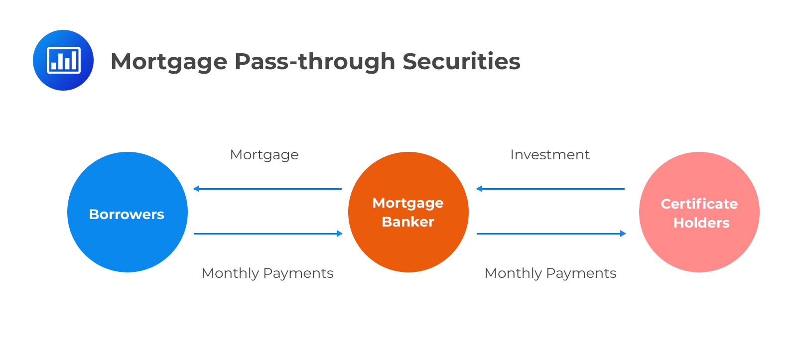Unlike covered bonds, mortgage pass-through securities are off-balance-sheet securitizations where investors receive cash flows based entirely on the performance of a pool. Payments are made to security holders each month from a servicer. These cash flows are usually reduced by the “service and other administrative fees” of the mortgages. A large percentage of pass-throughs carry implicit or explicit guarantee of performance, making default risk less of a concern to an investor. The main risk arises from prepayment, where the homeowner returns the principal earlier than scheduled. Prepayment implies that the investor loses out on interest that would be paid on that part of the principal.

Collateralized Mortgage Obligations

A collateralized mortgage obligation (CMO) is a fixed income security that uses mortgage-backed securities as collateral. CMOs are subdivided into tranches that vary in interest and risk based on the maturity structure of the mortgages. These tranches can have short or long maturities, cash flows that are fixed or floating, and other conditions. The most common payment structure is the waterfall mechanism (also called sequential pay) in which the tranches are ordered, with “Class A” receiving all principal repayments from the loan until it is retired, then “Class B,” and so on. The senior tranches carry less prepayment risk than a pass-through, while the lower ones bear more.

Collateralized mortgage obligations offer investors an opportunity to profit from a diversified, and therefore risk-reduced, set of mortgage-backed securities.

Structured Credit Products

Structured credit products work much like CMOs: they are backed by credit-risky loans or bonds and are split into tranches that have different degrees of credit risk. However, they introduce a new innovation – a sequential distribution of losses.

The most junior tranches lie first “in the line of fire” as they bear the first losses and are most likely to be written down. More senior tranches only begin to bear credit risk losses once the junior tranches have been written down to zero. As such, the most senior tranche has the highest credit rating and the lowest probability of writedowns.

In some cases, structured credit products can combine sequential distribution of losses with sequential payment technology as applied in CMOs to form complex products.

Collateralized Debt Obligations (CDOs)

CDO are Securitizations that repackage other securitizations. They may come in the form of a bond issued against a collateral pool consisting of ABS, MBS, or CLOs), collateralized mortgage obligations (CMOs), or collateralized bond obligations.

Structured credit products are usually set up as special purpose entities (SPE) or vehicles (SPV), also known as a trust. An SPE/SPV is intended to separate assets and liabilities of the structured product from those of the original creditors (originators) and of the servicer. An SPV/SPE often has a predefined purpose and legal identity. If the originator goes bankrupt, the assets sold to the SPV/SPE are not at risk. For this reason, the SPV/SPV is said to be bankruptcy-remote.

Tranching and Distribution of Losses in a Securitization

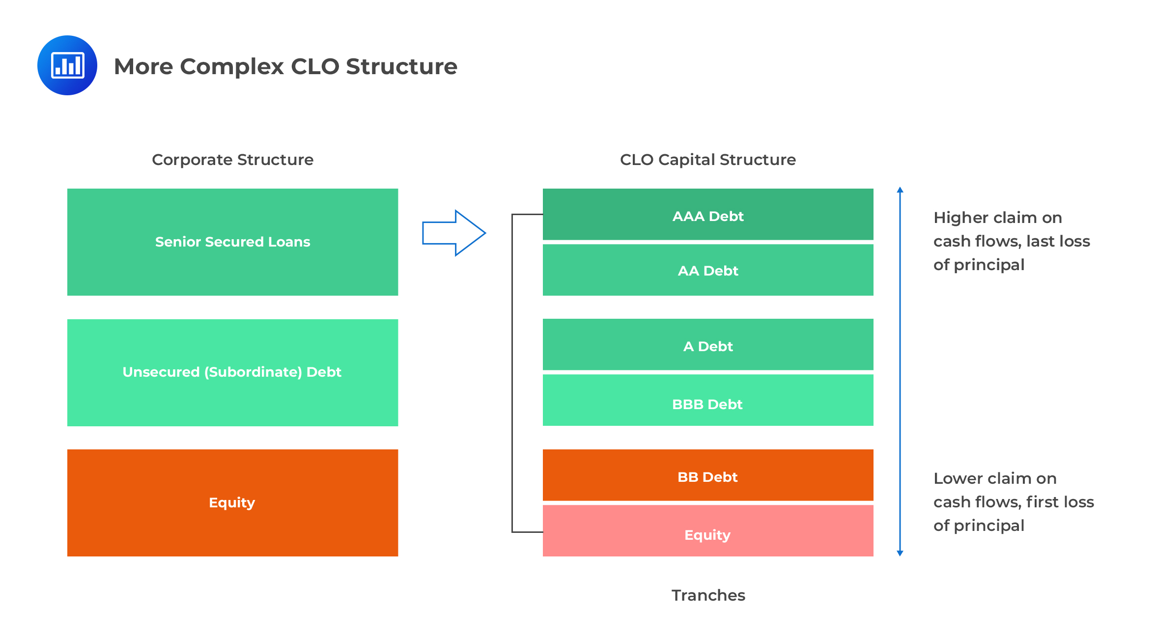
As noted earlier, most structured products have a sequential capital structure with different tranches.

$$ \begin{array}{c|c} \textbf{Assets} & \textbf{Liabilities} \\ \hline {} & \text{Senior Debt} \\ {{\text{Underlying Debt Instruments}}} & \text{Mezzanine debt} \\ {} & \text{Equity} \\ \hline \end{array} $$

The safest tranche is also known as the senior tranche. It offers the lowest interest rate, but it’s the first to receive cash flows from the underlying asset portfolio.

The middle (mezzanine) tranche offers a slightly higher interest rate and ranks just below the senior tranche. It takes the second spot during cash flow distribution. It absorbs losses only after the equity tranche is completely written down. The boundary between the senior tranche and the mezzanine tranche, expressed as a percentage of the total liabilities, is called the attachment point of the more senior tranche and the detachment point of the junior (mezzanine) tranche. The equity tranche only has a detachment point, and the most senior only has an attachment point.

The most junior tranche, also called the equity tranche, offers the highest interest rate (or high spread if the claim is floating) but ranks last during cash flow distribution. It’s also the first tranche to absorb any loss that may be incurred. The amount available for distribution to the equity (junior) tranche is whatever is left from the two other tranches less management fees. These fees can range from 0.5% to 1.5% annually.

The part of the capital structure below a given tranche is called its subordination or credit enhancement. We can interpret it as the fraction of the collateral pool that must be lost before the tranche takes any loss. As such, credit enhancement is greater for more senior bonds in the structure.

In general, credit enhancement (CE) takes two forms – internal CE or external CE. Internal CE may result from over-collateralization or excess spread.

Over-collateralization (OC) is the provision of collateral that is worth more than enough to cover claims from investors. In other words, the assets underlying a product have a value that’s in excess of the face value of securities issued to investors.

Excess spread is the difference between the cash flows collected and the payments made to all bondholders. For instance, let the interest rate received on the underlying collateral be 11%, and the coupon on the issued structured security be 10% (including fees). In this case, the excess spread is 1%. The excess spread is a built-in margin of safety that protects the pool (and originator) from losses. Its presence can actually improve the ratings on the structured product being assembled and make the resulting security more attractive to investors.

Investors in these tranches can protect themselves from default by purchasing credit default swaps. These CDS guarantee a pre-specified compensation in the event that a given tranche defaults. In turn, investors must make regular payments to the credit protection seller (writer of the CDS).

Each tranche is assigned its own credit rating, except the equity tranche. For instance, the senior tranche is constructed to receive an AAA rating. Highly rated tranches are sold to investors, but the junior-ranking ones may end up being held by the issuing bank. That way, the bank has an incentive to monitor the underlying loans.

Waterfall Structure in a Securitization

The waterfall structure has much to do with the rules about how the cash flows from the collateral are distributed to various securities in the capital structure. A typical structured credit product begins life with a certain amount of hard over-collateralization, since part of the capital structure is an equity note, and the debt tranches are less than 100 percent of the deal. Soft over-collateralization mechanisms may begin to pay down the senior debt over time with part of the collateral pool interest or divert part of it into a reserve that provides additional credit enhancement for the senior tranches.

Example: Waterfall Structure

A collateralized loan obligation is comprised of 100 identical leveraged loans with a par value of $1,000,000 each, priced at par. The loans pay a fixed spread of 4% over one –month LIBOR. The capital structure consists of equity, and a junior and a senior bond. Determine the excess spread, assuming that there are no defaults in the collateral pool.

Assumptions:

• The swap curve (“Libor”) is flat at 5%.
• There are no upfront, management, or trustee fees.
• The loans in the collateral pool and the liabilities are assumed to have a maturity of five years.
• All coupons and loan interest payments are annual and occur at year-end.
• There are no defaults in the collateral pool.

$$ \textbf{Loan and Tranche Information} $$

$$ \begin{array}{c|c|c} \textbf{B/S component} & \textbf{Par value} & \textbf{Coupon} \\ \hline \textbf{Assets} & {$100,000,000} & \textbf{ Libor} { + 4\%} \\ \hline \textbf{Liabilities} & {} & {} \\ \hline \text{Equity note} & {$5,000,000} & {} \\ \hline \text{Junior tranche} & {$10,000,000} & \text{ Libor}{ + 500} \text{ bps} \\ \hline \text{Senior tranche} & {$85,000,000} & \text{ Libor} {+ 50} \text{ bps} \\ \end{array} $$

Solution

From the data, we can see that the junior bond has a much wider spread than that of the senior bond and much less credit enhancement; the mezzanine/junior tranche attachment point is 5 percent, and the senior attachment point is 15 percent.

The annual cash flows will be as follows:

$$ \textbf{Tranche Interest Information} $$

$$ \begin{array}{c|c|c|c} {} & \textbf{Libor + Spread} & \textbf{Principal amount} & \textbf{Annual interest} \\ \hline \text{Collateral } & {0.05 + 0.04} & {$100,000,000} &{$9,000,000} \\ \hline \text{mezzanine} & {0.05 + 0.05} & { $10,000,000} & {($1,000,000)} \\ \hline \text{senior} & {0.05 + 0.005} & { $85,000,000} & {($4,675,000)} \\ \hline {} & {} & \text{Excess spread} & {$3,325,000} \\ \end{array} $$

Ideally, therefore, holders of the equity tranche would receive $3,325,000. However, the actual amount received is likely to be much less because of several reasons. To start with, cash flows to the equity tranche may be subject to an overcollateralization trigger where the maximum amount the tranche can receive is specified and any excess cash flows channeled to a trust account. Besides, cash flows will be lower if defaults occur.

To illustrate this, let’s go back to our example and assume that the default rate is 5% per year. That implies that on average, about 5 loans will default over the year. In this case, the total cash inflow from collateral will be $8,550,000 [= $100,000,000 * 0.09 *(1 – 0.05)]. There will still be sufficient cash to pay senior and junior bondholders in full. However, the cash flows into the equity tranche will be reduced.

$$ \textbf{Tranche Interest Information Assuming 5% Annual Default Rate} $$

$$ \begin{array}{c|c|c|c} {} & \textbf{Libor + Spread} & \textbf{Principal amount} & \textbf{Annual interest} \\ \hline \text{Collateral } & {0.05 + 0.04} & { $95,000,000} &{$8,550,000} \\ \hline \text{mezzanine} & {0.05 + 0.05} & { $10,000,000} & {($1,000,000)} \\ \hline \text{senior} & {0.05 + 0.005} & { $85,000,000} & {($4,675,000)} \\ \hline {} & {} & \text{Excess spread} & {$2,875,000} \\ \end{array} $$

The assumption that all the loans and bonds have precisely the same maturity date is only to simplify the process. In practice, however, there can be more than a dozen tranches with different coupon rates and maturities. Each of these tranches is rated.

Key Participants in the Securitization Process and Possible Conflicts of Interest

Loan Originator

A loan originator is the original lender who creates the debt obligations in a collateral pool. This is oftentimes, a bank. A good illustration of this is when the underlying collateral consists of bank loans or credit card receivables. Note, however, that a loan originator can also be a specialty finance company or mortgage lender. If most of the loans have been originated by a single intermediary, the originator may be called the sponsor or seller.

Underwriter

The underwriter is the financial engineer behind the securitization structure and is at times called the arranger. The underwriter is mostly, but not always, a large financial intermediary. Typically, the underwriter aggregates the underlying loans, and designs the securitization structure, including things such as the coupon rates, tranche sizes, and triggers. In this capacity, the underwriter is also the issuer of the securities. You may also come across a somewhat technical legal term – the depositor – being used to describe the issuer. The underwriter bears warehousing risk, the risk that the deal will not be completed and, consequently, the value of the accumulated collateral still on its balance sheet falls.

Rating Agencies

Rating agencies help investors to assess the riskiness of investments by assigning credit ratings to the various tranches engineered. Attachment points and the subordination structure are key cogs in the rating process. When companies are planning to issue a non-securitized bond, rating agencies have little influence over creditworthiness and are not involved in the structuring process. When issuing securitizations, however, rating agencies are usually more engaged in the structuring process and do more than just opining on creditworthiness.

A potential conflict of interest arises from the fact that rating agencies are compensated by the originators. The agencies may, therefore, be faced with a situation where they feel obliged to provide a favorable rating even when there are serious issues regarding the creditworthiness of a structure. The fact that the agencies are actively involved in designing the securitization structure only serves to exacerbate the potential conflict of interest. The agencies may dictate the amount of enhancement required to guarantee an investment-grade rating. Investors can cope with the potential conflict of interest by carrying out their own credit review of the deal or even demanding a wider spread.

Although the ratings under a securitization structure may be based entirely on the credit quality of a pool and the liability structure, they may also reflect any performance guarantees typically provided by monoline insurance companies. The insurer guarantees timely repayment of bond principal and interest in exchange for insurance premiums.

Servicers and Managers

A servicer collects principal and interest from loans in a collateral pool and disburses principal and interest to liability holders, as well as fees to the underwriter and itself. Servicers may also be actively involved in the monitoring of the collateral pool. If a loan in the pool is in distress, for example, the servicer may have the authority to evaluate possible options, including extending the term of the loan or foreclosing. Servicers, therefore, are firmly in the mix when it comes to conflict of interest between themselves and bondholders, or, between different classes of bondholders. Equity holders are often keen to have all loans perform to maturity because they are first in line to absorb any eventual loss. Therefore, they will be open to any arrangement that can help the borrower to see out the contract, including extending maturity. Senior bondholders, on the other hand, are less concerned with the possibility of default, especially, if the historical default rate is low such that there’s a very small chance that the senior tranche will make a loss.

Nonetheless, any loan extension may avert immediate loss but increase the potential future loss, thereby increasing the riskiness of the bond as a whole and eroding credit enhancement. At any one time, the servicer takes action that is more favorably aligned to the interests of some bondholders than of others.

When the collateral pool is actively managed, the manager may not be so keen to monitor its financial health if there’s no incentive to do so. To mitigate conflict of interest, the structure may be designed in such a way that the originator or manager bears the first loss in the capital structure.

Credit Scenario Analysis of a Securitization

Let’s revisit our example above where the excess spread (after paying senior and mezzanine tranche bondholders) was $3,325,000.

$$ \textbf{Tranche Interest Information} $$

$$ \begin{array}{c|c|c|c} {} & \textbf{Libor + Spread} & \textbf{Principal amount} & \textbf{Annual interest} \\ \hline \text{Collateral } & {0.05 + 0.04} & { $100,000,000} &{$9,000,000} \\ \hline \text{mezzanine} & {0.05 + 0.05} & { $10,000,000} & {($1,000,000)} \\ \hline \text{senior} & {0.05 + 0.005} & { $85,000,000} & {($4,675,000)} \\ \hline {} & {} & \text{Excess spread} & {$3,325,000} \\ \end{array} $$

Instead of channeling the entire amount into the pockets of equity holders, originators will often divert part of it to an excess spread account, also known as a trust/over-collateralization account.

The aim is to create further protection for the senior and mezzanine tranches by creating an alternative pool of funds that can be used to make payments to investors in case interest from the collateral pool proves insufficient. In other words, the funds in the over-collateralization account will be used to pay interest on the bonds if there is not enough interest flowing from the loans in the collateral pool. Any built-up funds in the over-collateralization account at maturity will be released to equity holders. The funds in the over-collateralization account earn interest at the money market rate.

The over-collateralization account (we will denote this as OA) creates a reliable buffer, especially when the default rate is low. Unless the default rate is very high, there will be some cash inflow into the account every year.

Let’s make two more assumptions:

1. Loans in the collateral pay no interest if they have defaulted at any time during the prior year. That means that there is no partial interest; interest is paid at the end of the year by surviving loans only.
2. In the event of default, the recovery rate is 40%, and all recovered monies are channeled into the over-collateralization account where accumulation occurs at the money market rate.

Notation

N = Number of loans in initial collateral pool (in our case, N = 100).

\({\text{d}}_{\text{t}}\) = Number of defaults in the course of year t.

\({\text{L}}_{\text{t}}\) = Aggregate loan interest received by the trust at the end of year t.

B = Total coupon (interest) due to both the junior and senior bonds (in our example above, B = $5,675,000 for all t).

K = Maximum amount diverted from excess spread into the overcollateralization account at the end of year t.

\({\text{OC}}_{\text{t}}\) = Amount actually diverted from excess spread into the overcollateralization account at the end of year t.

\({\text{R}}_{\text{t}}\)= Recovery amount deposited into the overcollateralization account at the end of year t.

r = Money market rate assumed to be constant (We will assume r = 5%).

To determine the cash flow to equity, we will ask ourselves the following question:

Q: Is the excess spread positive?

In notations, we are simply asking: is \({\text{L}}_{\text{t}}-\text{B}≥0\)?

If yes:

A further test must be performed to determine how much flows into the OA: is \({\text{L}}_{\text{t}}-\text{B} \ge {\text K}?\). If yes, then K is channeled into the OA, and \(\text{L}_{\text{t}}-\text{B}-\text{K}\), flows to equity holders: \({\text{OC}}_{\text{t}}=\text{K}\). If no, then the entire amount \({\text{L}}_{\text{t}}-\text{B}\) is channeled into the OA, and equity holders receive nothing: \({\text{OC}}_{\text{t}}\)=\({\text{L}}_{\text{t}}-\text{B}\).

If No:

If the excess spread is not positive, then the interest is not sufficient to pay bondholders and all \({\text{L}}_{\text{t}}\) goes to bondholders. The shortfall, therefore, is \(\text{B}-{\text{L}}_{\text{t}}\).

In this scenario, the next step is to check if the OA has accumulated an amount that can cover the shortfall. If the OA has enough funds, bondholders are paid in full. If the OA does not have enough, the bondholders suffer a writedown.

Now, let’s see how a positive default rate affects cash flows. First, let’s assume that the number of defaults, \({\text{d}}_{\text{t}}\) is constant in any given year, and the recovery rate in year t is 40%. In this case, the recovery amount deposited into the over-collateralization account at the end of year t, \({\text{R}}_{\text{t}}\) is calculated as follows:

$$ {\text{R}}_{\text{t}}=0.4{\text{d}}_{\text{t}} \times \text{loan amount} $$

Therefore, the total amount deposited into the trust account in year t is:

$$ {\text{R}}_{\text{t}}+ {\text{OC}}_{\text{t}} \quad \text{t}=1,…\text T-1 $$

The value of the overcollateralization account at the end of year t, including the cash flows from recovery and interest paid on the value of the account at the end of the prior year, is:

$$ { { \text{R} } }_{ { \text{t} } }+{ { \text{OC} } }_{ { \text{t} } }+\sum _{ \tau =1 }^{ \text{t}-1 }{ { \left( 1+\text{r} \right) }^{ \text{t}-\tau } } { { \text{OC} } }_{ { \text{t} } } \quad \text{t}=1,…\text{T}-1 $$

If the excess spread is negative, i.e.,\({\text{L}}_{\text{t}}-\text{B}\) < 0, the custodian must check if the OA has an amount that is enough to cover the shortfall. Formally, the test is as follows:

$$ { { \text{R} } }_{ { \text{t} } }+\sum _{ \tau =1 }^{ \text t-1 }{ { \left( 1+\text{r} \right) }^{ \text{t}-\tau } } { { \text{OC} } }_{ { \text{t} } }>\text{B}-{ { \text{L} } }_{ { \text{t} } } $$

Note that we do not have \({ { \text{OC} } }_{ { \text{t} } }\) to add to \({ { \text{R} } }_{ { \text{t} } }\) in the equation above because there is no excess spread in the current period.

If the test is true, then the bondholders are paid in full. If not, then the OA is literally swept clean and all of its holdings channeled to bondholders. In this case, they receive

$$ { { \text{R} } }_{ { \text{t} } }+ \sum _{ \tau =1 }^{ \text{t}-1 }{ { \left( 1+\text{r} \right) }^{ \text{t}-\tau } } { \text{OC} }_{ \text{t} } \text{ from the OA} $$

The amount to be diverted in any year t is given by:

$$ { { \text{ OC } } }_{ { \text{t} } }=\left\{ \begin{matrix} \text{min}\left( { { \text{ L } } }_{ { \text{ t } } }-\text{ B,K } \right) \\ \text{ max }\left[ { { \text{ L } } }_{ { \text{ t } } }-\text{ B }=\left( \sum _{ \tau =1 }^{ \text{ t }-1 }{ { \left( 1+\text{ r } \right) }^{ \text{ t }-\tau } } { { \text{ OC } } }_{ { \text{t} } }+{ { \text{ R } } }_{ { \text{t} } } \right) \right] \end{matrix} \right\} \text{for}\left\{ \begin{matrix} { { \text{ L } } }_{ { \text{t} } }\ge \text{ B } \\ { { \text{ L } } }_{ { \text{t} } } < \text{ B } \end{matrix} \right\} $$

Once we have established how much excess spread, if any, flows into the OA at the end of year t, we can determine how much cash flows to equity holders at the end of year t. The equity cash flow is

$$ \text{max}\left( { { \text{L} } }_{ { \text{t} } }-{\text{B}}-{ { \text{OC} } }_{ { \text{t} } },0\right) \quad \text{t}=1,…\text T-1 $$

In the terminal year, cash flows are examined separately for several reasons:

1. All the surviving loans up to that point reach maturity and principal is returned.
2. There is no diversion to the OA because the structure ends. All proceeds have to be shared.
3. Since there is no diversion to the OA, there’s no need to test overcollateralization triggers.

The equations below summarize terminal cash flows:

Loan interest=\(\left( \text{ N }-\sum _{ \text{t}=1 }^{ \text{T} }{ { \text{d} }_{ \text{t} } } \right) \times \left( \text{ Libor+spread } \right) \times \text{ par }\)

Proceeds from redemption of all surviving loans=\(\left( \text{ N }-\sum _{ \text{t}=1 }^{ \text{T} }{ { \text{d} }_{ \text{t} } } \right) \times \text{ par }\)

Recovery \(\text{R}_{ \text{t} }=0.4\text{d}_{ \text{t} }\times \text{par}\)

Residual in OA account = \(\sum _{ \tau =1 }^{ \text{t}-1 }{ { \left( 1+\text{r} \right) }^{ \text{t}-\tau } } \text{OC}\)

In the terminal year, therefore, the waterfall mechanism takes full effect: If the sum of all terminal cash flows is large enough, the senior tranche is paid off. The remainder, if any, is used to pay off the junior tranche, and any remainder flows to equity. Sometimes there may be no cash flows left for equity holders after paying off the junior tranche, especially if the default rate has been high.

Examples: Equity IRR Given Different Default Rates

$$ \textbf{Cash flow structure Given a Constant Default Rate of 2%} $$

$$ \begin{array}{l|c} \textbf{Assumptions and Notation} & \textbf{Values} \\ \hline \text{Number of loansin the pool at t = 0} & \text{100} \\ \text{Default rate} & \text{2% (constant)} \\ \text{Bond coupon interest due, B (in millions)} & \text{\$5.675} \\ \text{Maximum amount diverted, K (in millions)} & \text{\$2.00} \\ \text{Recovery rate} & \text{40%} \\ \text{Money market rate} & \text{5%} \\ \text{Aggregate loan interest, L(t)} & \text{9% (5% Libor + 4% Spread)} \\ \end{array} $$

$$ \begin{array}{l|c|c|c|c|c|c} \textbf{t} & \textbf{0} & \textbf{1} & \textbf{2} & \textbf{3} & \textbf{4} & \textbf{5} \\ \hline \text{Defaults, d(t), rounded} & \text{} & \text{2} & \text{2} & \text{2} & \text{2} & \text{2} \\ \text{Cumulated Defaults} & \text{} & \text{2} & \text{4} & \text{6} & \text{8} & \text{10} \\ \text{Survived} & \text{} & \text{98} & \text{96} & \text{94} & \text{92} & \text{90} \\ \text{Loan interest, L(t)} & \text{} & \text{\$8.82} & \text{\$8.64} & \text{\$8.46} & \text{\$8.28} & \text{\$98.10} \\ \text{Excess spread, L(t) – B} & \text{} & \text{\$3.15} & \text{\$2.97} & \text{\$2.79} & \text{\$2.61} & \text{} \\ \text{Overcollateralization, OC(t)} & \text{} & \text{\$2.00} & \text{\$2.00} & \text{\$2.00} & \text{\$2.00} & \text{} \\ \text{Recovery, R(t)} & \text{} & \text{\$0.80} & \text{\$0.80} & \text{\$0.80} & \text{\$0.80} & \text{\$0.80} \\ \text{OC + Rec, OC(t) + R(t)} & \text{} & \text{\$2.80} & \text{\$2.80} & \text{\$2.80} & \text{\$2.80} & \text{} \\ \text{Equity flow} & \text{-5} & \text{\$1.15} & \text{\$0.97} & \text{\$0.79} & \text{\$0.61} & \text{\$10.91} \\ \text{Results} & \text{} & \text{Y} & \text{Y} & \text{Y} & \text{Y} & \text{} \\ \text{OC a/c} & \text{} & \text{\$2.80} & \text{\$5.74} & \text{\$8.83} & \text{\$12.07} & \text{\$12.68} \\ \text{Equity IRR} & \text{} & \text{\$1.15} & \text{\$0.97} & \text{\$0.79} & \text{\$0.61} & \text{\$10.91} \\ \end{array} $$

$$ \begin{array}{l|c|c} \text{Total terminal cash flows = L(5) + R(5) + OC a/c} & \text{\$111.58} & \text{IRR: 29.79%} \\ \hline \text{Amount owed to bond tranches = \$85 + \$10 + \$5.675} & \text{\$100.68} & \text{} \\ \hline \text{Equity terminal cash flow} & \text{\$10.91} & \text{} \\ \end{array} $$

With a constant default rate of 2%, the figure above shows that the equity tranche generates an IRR of approx. 29.79%. However, increasing the default rate to 8%, as illustrated in the example below, generates a negative IRR for equity. The excess spread declines over time as defaults pile up.

$$ \textbf{Cash flow structure Given a Constant Default Rate of 8%} $$

$$ \begin{array}{l|c} \textbf{Assumptions and Notation} & \textbf{Values} \\ \hline \text{Number of loansin the pool at t = 0} & \text{100} \\ \text{Default rate} & \text{8% (constant)} \\ \text{Bond coupon interest due, B (in millions)} & \text{\$5.675} \\ \text{Maximum amount diverted, K (in millions)} & \text{\$2.00} \\ \text{Recovery rate} & \text{40%} \\ \text{Money market rate} & \text{5%} \\ \text{Aggregate loan interest, L(t)} & \text{9% (5% Libor + 4% Spread)} \\ \end{array} $$

$$ \begin{array}{l|c|c|c|c|c|c} \textbf{t} & \textbf{0} & \textbf{1} & \textbf{2} & \textbf{3} & \textbf{4} & \textbf{5} \\ \hline \text{Defaults, d(t), rounded} & \text{} & \text{8} & \text{7} & \text{7} & \text{6} & \text{6} \\ \text{Cumulated Defaults} & \text{} & \text{8} & \text{15} & \text{22} & \text{28} & \text{34} \\ \text{Survived} & \text{} & \text{92} & \text{85} & \text{78} & \text{72} & \text{66} \\ \text{Loan interest, L(t)} & \text{} & \text{\$8.28} & \text{\$7.65} & \text{\$7.02} & \text{\$6.48} & \text{\$71.94} \\ \text{Excess spread, L(t) – B} & \text{} & \text{\$2.61} & \text{\$1.98} & \text{\$1.35} & \text{\$0.81} & \text{} \\ \text{Overcollateralization, OC(t)} & \text{} & \text{\$2.00} & \text{\$1.98} & \text{\$1.35} & \text{\$0.81} & \text{} \\ \text{Recovery, R(t)} & \text{} & \text{\$3.20} & \text{\$2.80} & \text{\$2.80} & \text{\$2.40} & \text{\$2.40} \\ \text{OC + Rec, OC(t) + R(t)} & \text{} & \text{\$5.20} & \text{\$4.78} & \text{\$4.15} & \text{\$3.21} & \text{} \\ \text{Equity flow} & \text{-5} & \text{\$0.61} & \text{\$0.00} & \text{\$0.00} & \text{\$0.00} & \text{} \\ \text{Results} & \text{} & \text{Y} & \text{Y} & \text{Y} & \text{Y} & \text{} \\ \text{OC a/c} & \text{} & \text{\$5.20} & \text{\$10.24} & \text{\$14.90} & \text{\$18.86} & \text{\$19.8} \\ \text{Equity IRR} & \text{} & \text{\$0.61} & \text{\$0.00} & \text{\$0.00} & \text{\$0.00} & \text{\$0.00} \\ \end{array} $$

$$ \begin{array}{l|c|c} \text{Total terminal cash flows = L(5) + R(5) + OC a/c} & \text{\$94.14} & \text{IRR: -87.80%} \\ \hline \text{Amount owed to bond tranches = \$85 + \$10 + \$5.675} & \text{\$100.68} & \text{} \\ \hline \text{Equity terminal cash flow} & \text{\$0.00} & \text{} \\ \end{array} $$

As defaults pile up, the most dramatic cash flow changes occur in the equity tranche. At a low default rate, the equity continues to receive at least some cash almost throughout the life of the securitization. But as the default rate increases, interim cash flows to the equity terminate much earlier. 

Computing and Evaluating Interim Cashflows in a Three-Tiered Securitization Structure

Understanding the Securitization Structure

In a three-tiered securitization structure, cash flows from the underlying assets are distributed to various debt tranches and an equity component based on a pre-determined set of rules referred to as the waterfall. The debt is typically structured into senior, mezzanine (junior), and equity notes, with each one providing a different level of credit enhancement and risk exposure to investors.

Initial Setup Example

For our example, consider a pool of 100 leveraged loans each worth $1 million for a total value of $100 million at a floating interest rate of LIBOR plus 3.5% (350 basis points). The securitized liabilities are divided into:

• Equity Note: $5 million
• Mezzanine (Junior) Debt: $10 million, returning LIBOR plus 5.0% (500 basis points)
• Senior Debt: $85 million, returning LIBOR plus 0.5% (50 basis points)

The credit enhancement for the mezzanine debt is equivalent to the size of the equity tranche. For the senior bond, the enhancement is the sum of the equity and mezzanine tranches. Initially, there is no overcollateralization present.

If we assume no defaults in the collateral pool and LIBOR remains a flat 5%, the annual cash flows can be computed as follows:

For the Collateral Pool (Total Principal $100 million)

• Interest Rate: LIBOR + 3.5% (350 basis points)
• Annual Cash Flow: (0.050 + 0.035) × $100,000,000 = $8,500,000

For the Mezzanine Debt (Principal $10 million)

• Interest Rate: LIBOR + 5.0% (500 basis points)
• Annual Cash Flow: (0.050 + 0.050) × $10,000,000 = $1,000,000

For the Senior Debt (Principal $85 million)

• Interest Rate: LIBOR + 0.5% (50 basis points)
• Annual Cash Flow: (0.050 + 0.005) × $85,000,000 = $4,675,000

The excess spread, in a no-default scenario, is the remaining cash flow after servicing the mezzanine and senior debt:

Total Collateral Cash Flow – (Mezzanine Debt Service + Senior Debt Service) = $8,500,000 – ($1,000,000 + $4,675,000) = $2,825,000.

Evaluating Interim Cashflows

Absent any defaults, the excess spread may be allocated to cover potential losses, added to credit support, or distributed to equity note-holders. The excess spread shields the tranches from default risk, improving their credit quality.

In a default scenario, the incoming cash flow is reduced, affecting the distribution across the tranches. Losses are typically absorbed in a sequential order, starting with equity, followed by mezzanine, and finally, the senior tranche.

Timely payments and managing the excess spread are crucial for maintaining the integrity of the securitization structure and securing the interim cash flows for the tranches. This entails a strong grasp of structuring cash flows, especially in the face of defaults, which is a critical skill set for financial risk managers in the structured credit market.

Treatment of Excess Spread in a Securitization Structure and Overcollateralization Account Estimation

Overcollateralization Mechanism

In the context of a securitization structure, the treatment of the excess spread—defined as the spread between the interest received from the collateral pool and the interest paid out to the debt tranches—can be multifaceted. A common approach is to use a portion of the excess spread for overcollateralization purposes, strengthening the credit support within the structure.

For example, an overcollateralization mechanism can be introduced whereby up to $1,150,000 of the excess spread is diverted annually to an overcollateralization account. This account is akin to a reserve account earning the financing or money market rate. If the excess spread is below this threshold, the entire amount is funneled into the account; if it exceeds it, the excess over $1,150,000 is paid to equity.

The funds in the overcollateralization account serve a pivotal role. They are primarily used to cover interest payments on the bonds if there is insufficient cash flow from the collateral loans in any given period. Remaining funds are earmarked for distribution to the equity tranche but only at the very end of the securitization’s life.

Recoveries and Defaults

For loans that default within the collateral pool, it is assumed no interest is paid by these loans for that year—defaulted loans contribute no interest to the annual cash flows. Moreover, it is assumed that a default will result in a recovery rate of 40 percent, with the recovered amount being deposited into the overcollateralization account.

The treatment of recoveries is structured to protect the more senior tranches—in a more complex or real-world structuring these funds might be distributed directly to senior or mezzanine bondholders. In our simplified scenario, we “escrow” such recoveries, placing them in the overcollateralization account to be used similarly to excess spread funds—first to cover interest and then to increase credit support.

Estimating the Value of the Overcollateralization Account

To estimate the value of the overcollateralization account at the end of each year, the following formula can be used:

\[ \text{Year-end value} = (\text{OC}_{t-1} + \text{Recoveries}_t) \times (1 + r) + \text{OC}_t \]

Where:

• \(\text{OC}_{t-1}\): Overcollateralization amount at the end of the previous year
• \(\text{Recoveries}_t\) Total recovery amount from defaults during year (t)
• \(r\): Money market or swap rate
• \(\text{OC}_t\): Amount diverted from the excess spread to the overcollateralization account at the end of year (t)

Excess Spread Tests for Overcollateralization and Equity Cash Flows

Overview of the Testing Process

The custodian of a securitization structure is responsible for conducting tests on the excess spread at the end of each year. The objective of these tests is to determine how the available excess spread should be allocated between the overcollateralization account and equity note holders. The tests form a two-step decision-tree process and can be described as a sequence of if-then conditions based on scenarios concerning the amount of excess spread.

Step 1: Testing for Positive Excess Spread

This initial test verifies whether the excess spread is positive:

• If positive (Lr – B > 0): The surplus after bond coupon payments is determined. This surplus is the difference between the aggregate loan interest, Lr, and the bond coupon interest due, B.
• If the excess spread is enough to cover the maximum annual diversion to the overcollateralization account (i.e., if Lr – B ≥ K), then K is diverted to this account.
• If not (Lr – B < K), then the whole surplus (Lr – B) goes into the overcollateralization account, leaving no excess spread for equity note holders.
• Alternatively, if Lr – B equals zero, the entire excess spread goes to servicing bond payments, with no contribution to the overcollateralization account.

Step 2: Handling Negative Excess Spread

• If negative (Lr – B < 0): The shortfall needs to be managed. The custodian must then verify if the overcollateralization account and the recoveries from defaults in the past year are sufficient to cover this shortfall.

  • If the overcollateralization account balance plus recoveries (Rr) can cover the shortfall (i.e., the sum exceeds B – Lr), then the shortfall amount is paid from the overcollateralization account to cover bond payments.
  • If the funds are insufficient (the sum is less than B – Lr), the total amount available from the overcollateralization account and recoveries is utilized, depleting the account to cover as much of the bond payments as possible.

Equity Cash Flow Determination

After these tests have been conducted and the overcollateralization cash flow has been determined, the custodian then calculates the cash flows to the equity note holders. If there is a positive excess spread remaining after the overcollateralization account has been funded, this surplus is distributed to equity. However, if the excess spread is zero or negative, no cash flows to equity prior to the maturity of the securitization.

Illustration of Cash Flow Results in Practice

The described mechanism, when applied to default scenarios of 2.0 percent, 7.5 percent, and 10.0 percent, showcases varying results for the overcollateralization account depending on the magnitude of the defaults and the resultant excess spread. In low-default scenarios, cash flow to equity can be maintained throughout the life of the securitization, whereas in high-default scenarios, equity cash flows may cease earlier due to insufficient surplus. Recoveries that are hold back and not used to redeem bonds pre-maturity add to the complexity of the tests and the interpretation of resulting cash flows.

Through the yearly tests, the custodian ensures that the securitization structure is adhering to its waterfall payment agreements, protects senior bondholders, and determines the distribution of excess spread effectively between the overcollateralization account and equity note holders.

The Simulation Procedure and the Role of Correlation

In our calculations up to this point, we have made several assumptions, notably that the default rate is constant, and there’s no correlation between loans. In reality, the default rate is a random variable, and loans show some correlation.

We can estimate credit losses for the various tranches in a securitization structure by way of simulation, which allows us to change our initial assumptions.

Step 1: Estimate Parameters

The first step is to determine the parameters for the valuation, particularly, the probability of default for each security. We also need to determine the correlation that ties the securities together.

Step 2: Generate Default Time Simulations

Next, we need to simulate the default times of each security included in the collateral pool, using the estimated parameters and the copula approach. We simulate the default times of each security in the collateral pool.

Step 3: Compute the Credit Losses

Using the simulation results, (i.e., default probabilities and associated timings) we can simulate cash flows from the security pool in every period.

Effect of Default Probabilities and Default Correlations on the Credit Risk in a Securitization

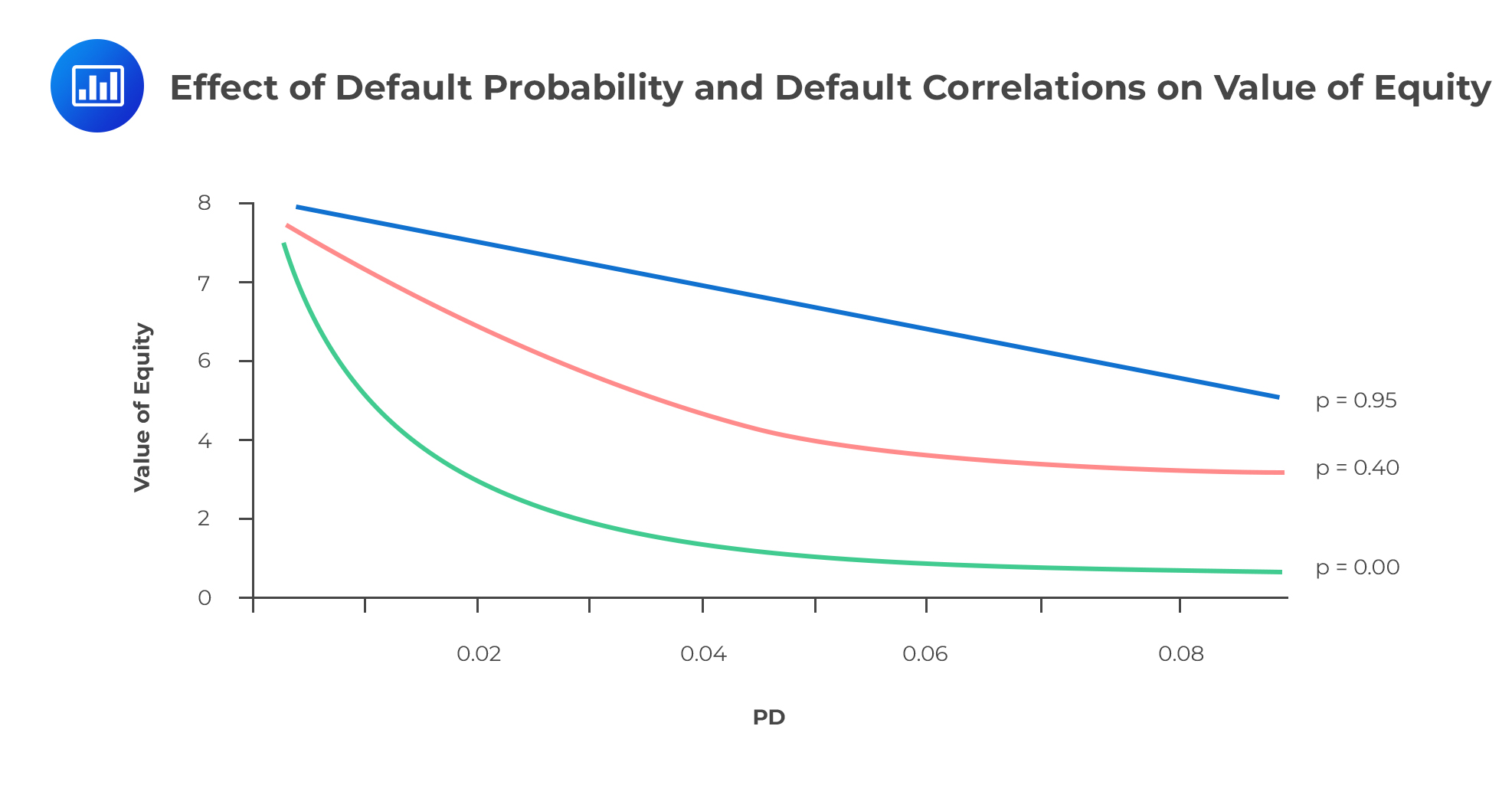
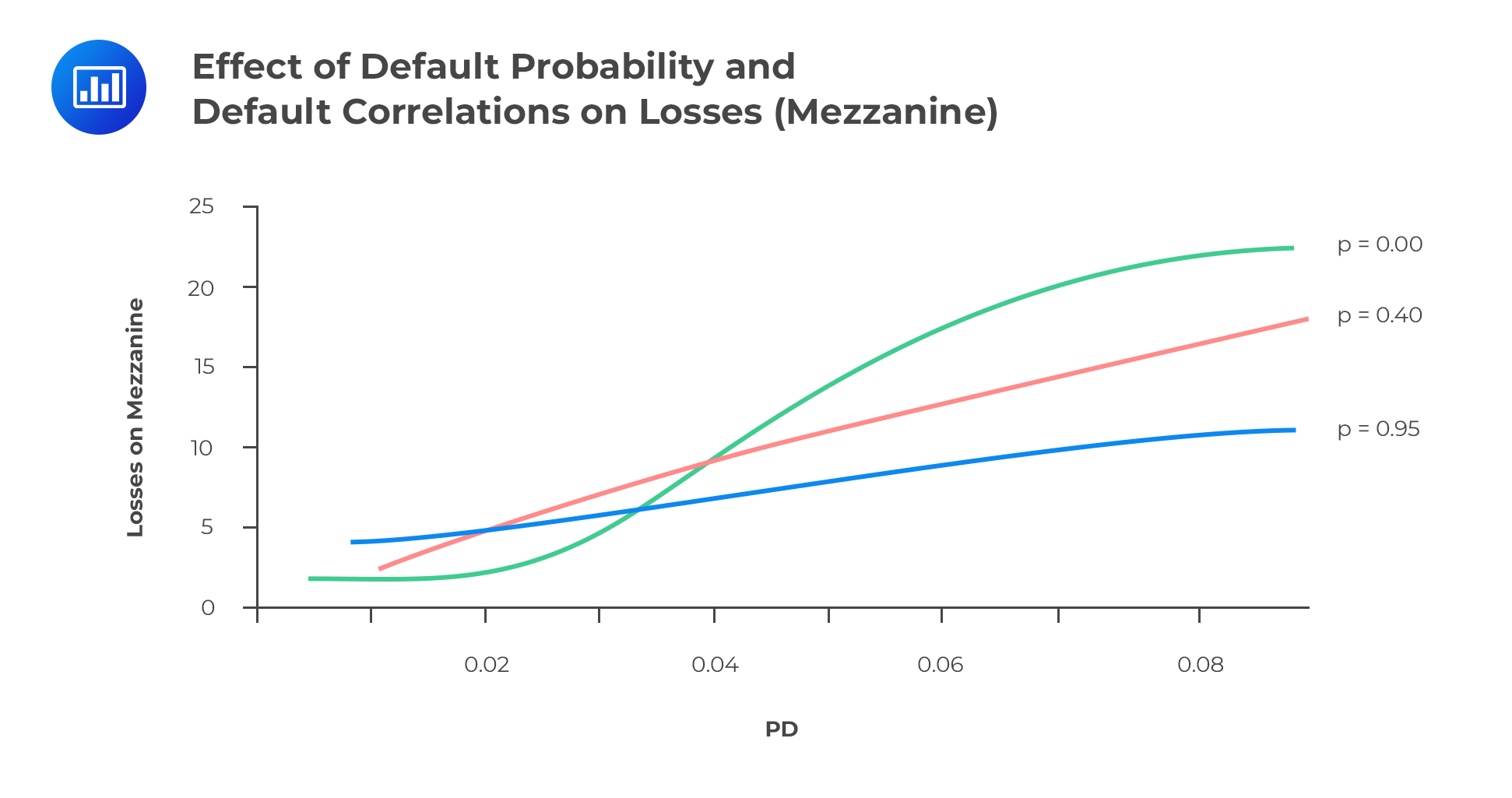
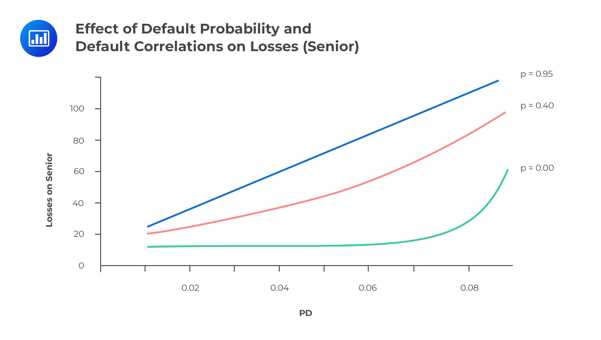
The interaction between default probability and default correlation has important implications on credit risk under a securitization framework.

An increase in the default rate hurts all the tranches in a securitization structure. It increases bond losses and decreases the equity IRR.

An increase in correlation, on the other hand, can bring about mixed results, depending on the level of default.

Equity Tranche

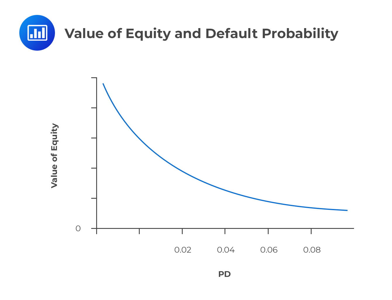
The equity value tends to exhibit positive convexity: As the default rate increases from a very low level, the effect on equity value is extremely huge. But as the default rate increases further and further from its low values, the responsiveness of the equity value drops off. We can use a bit of biological analogy here: If someone happens to physically assault you, the first few blows tend to be the most painful. Or better yet, the human body tends to be hit really hard by pathogens (disease-causing organisms) at the first time of the attack. As time goes by, the body is able to adapt and minimize the impact caused by a further onslaught of pathogens. Once you have lost most of your investment due to an increase in the default rate, you will be left with much less to lose following even more defaults in the future.

Mezzanine Trance

When the default rate is low, an increase in correlation increases the likelihood of losses to the mezzanine tranche (similar to the senior tranche). But when the default rate is high, an increase in correlation actually decreases the expected losses to the mezzanine tranche because of the increased likelihood of fewer defaults. In other words, mezzanine bonds behave more like the senior bonds at low default rates and more like the equity tranche when the default rates are high. We can also look at this differently: At low default rates, there’s a very small chance that the attachment point for mezzanine bonds will be broken. But at high default rates, a breach of the attachment point is highly likely.

Convexity presents yet another interesting perspective when it comes to default rates. Maybe to take you back to bond convexity a little bit, a bond that has positive convexity would typically experience larger price increases as yields fall but relatively smaller price decreases when yields increase.

Senior Tranche

At low correlations, senior bonds exhibit negative convexity: As defaults pile up, the decline in bond value increases. The mezzanine tranche is ambiguous. It exhibits negative convexity for low default rates and positive convexity for high default rates.

At high correlations, all bonds tend to shake off the convexity effect. They respond more linearly to an increase in default rates.

Measuring Default Sensitivities for Tranches

Let’s now look at the effect of the default on the various securitization tranches independently without tying everything to correlation. To do this, we will revive the concept of DV01.

default01. The default probability π is shocked up by 10 basis points and all tranches revalued. Then, the default probability is shocked down by 10 basis points and the tranches revalued yet again. The default01 is then computed as:

$$ \cfrac { 1 }{ 20 } \left[ \left( \text{mean value/loss for } \pi + 0.0010 \right) -\text{mean value/loss for } \pi – 0.0010 \right] $$

The default01 is computed for each combination of \(\pi\) and \(\rho \).

It can be shown that for all tranches, the default01 is positive, regardless of the values of \(\pi\) and correlation \(\rho \). This happens because equity and bond values decrease monotonically as the default probability rises. In addition, the default01 converges at zero for all tranches as the default rates increase. Once the losses are extremely high, the incremental impact of additional defaults is low.

Risk Factors That Impact Structured Products

The risk factors that impact structured products involve a combination of credit market dynamics, investor behavior, legal frameworks, and economic incentives, among other considerations. Understanding these factors is essential in the analysis and management of risks associated with structured credit products.

Incentives and Behavior of Loan Originators

Loan originators face certain incentives that can significantly impact the risk profile of structured products:

• Monitoring and Information Asymmetry: The challenge of evaluating and monitoring the credit quality of loans, often referred to as the “lemons” problem, suggests that originators may have incentive to securitize loans of lower quality than what is disclosed.
• Risk Retention: Retaining equity or other subordinated tranches, or a portion of the asset itself, can mitigate risks by aligning the originator’s interests with those of the senior tranche holders.
• Regulatory Consequences: The Dodd-Frank Act has acknowledged these conflicts of interest and is expected to restrict issuers from completely selling off all tranches, thereby necessitating some form of risk retention.

Legal Implications and Underwriting Standards

• Legal Representations: Structured products are affected by the legal representations made by the loan seller regarding the loans’ underwriting standards. Discrepancies in these standards can lead to legal recourses, impacting the stability of securitizations.

Investors’ Incentives and Behaviors

• Securitization Appeal: Securitization allows capital market investors to participate in loan pools often confined to banks, such as mortgages and auto loans, which adds a layer of risk due to investor unfamiliarity.
• Tranching Technology: Tranching can mitigate default risk for senior tranches but may increase exposure to systemic risk. Subordinate tranches can attract investors with a higher risk appetite.
• Demand for Yield: Institutional investors may undertake insufficient due diligence given their need to deploy large sums of capital while seeking returns that meet their targets, leading to an underestimation of systematic risks.
• Mezzanine Tranche Volatility: These tranches are complex as their behavior can range from resembling safe senior tranches to riskier equity tranches, leading to an uncertain investor base.

Economic and Regulatory Arbitrage

• Revenue Generation: Loan originators and issuers may be motivated to engage in securitization because the fees and the servicing role can be more profitable than retaining the loans.
• Capital Requirements: Securitization allows financial intermediaries to retain some exposure to a loan pool while significantly reducing the regulatory capital required.

Investment Vehicles and Funds

• Off-Balance Sheet Entities: Vehicles such as money market mutual funds that invest in securitizations can also impact the risk profile, given their role as significant investors.

Each of these factors plays a role in shaping the overall risk factors that impact structured credit products. They highlight the intricate web of motivations, behaviors, and external pressures that drive the securitization process and affect its stability and performance. Assessing these risks requires a thorough understanding of the entire securitization value chain—from originators to the end investors—as well as the economic environment in which these products are structured, sold, and traded.

Tranche Risk

1. Systematic Risk

   Even when the collateral pool is well-diversified, structured products tend to have quite high systematic risk. High systematic risk can be expressed through the presence of a high default correlation. If the default correlation is high, it means that there is a low but material probability of an unusually high number of defaults.

   As long as the correlation is high, all the tranches have a degree of systematic risk. There’s a likelihood of a large loss in the senior bond if the correlation is high.

   The degree of systematic risk is highly dependent on the securities making up the collateral pool and the level of credit enhancement.

2. Tranche Thinness

   In most securitization structures, the equity and junior tranches are relatively thin. In the examples we have used so far, the two tranches constituted just 15% of the collateral pool. This thinness manifests itself in VaR calculations. The 95% and 99% credit VaRs are quite close. This implies that if the two have been breached, there’s a high likelihood that the loss is very large.

3. Granularity

   The granularity of the collateral pool is a major indicator of the level of diversification. A collateral pool made up of a few large loans is riskier than another pool with many loans of smaller amounts.

Implied Correlation

If you recall, the implied volatility of an option contract refers to the value of the volatility of the underlying instrument which, when input into an option pricing model, will return a theoretical value equal to the current market price of the said option. The implied default correlation is a closely related concept: It is the value of the correlation built into the observable market prices of the various securitized tranches.

In essence, structured credit products are claims on cash flows of credit portfolios. Their prices, therefore, reflect an implied default correlation of those portfolios. Earlier on, we saw how to estimate the values of securitization tranches. In the same way, it is possible to reverse engineer the valuation process and use the market-observed prices of structured credit products and come up with a value of the default correlation.

The implied default correlation is a risk-neutral parameter that can always be estimated as long as there are observable prices of the portfolio credit products.

Issuer and Investor Motivations for Structured Credit

To identify why securitizations are created, incentives of the loan originators need to be identified.

Incentives of the issuers

1. Lower Cost of funding

   Securitization provides a cheaper funding method for the issuer. The interest rate payable to investors in securitized assets is much lower than that which the originator would have to pay if they issued a coupon bond of the same maturity as the securitized portfolio.

2. Exit Avenue

   Without securitization, the originator would either have to retain the underlying assets on the balance sheet or sell them in the secondary market. As such, securitization offers a good “exit” route, especially when the securitization costs much less than the next best alternative.

3. Arbitrage CDOs

   Sometimes, securitization may be designed to specifically capture the spread between the underlying loan interest and the coupon rates payable to investors.

4. Balance Sheet Relief

   Hiving a significant amount of loans off the balance sheet can come with benefits for the originator. Banks, for example, may be subject to lower regulatory capital requirements.

5. Fees

   A sponsor may make more money from originating and possibly servicing loans than retaining them on the balance sheet.

Incentives of Investors

1. A Unique Investment Opportunity

   Securitization allows investors to have more direct legal claims on loans and portfolios of receivables. Capital market investors are able to participate in diversified loan pools in sectors that would otherwise be the preserve of banks alone. These include mortgages, credit card receivables, and automobile loans.

2. Risk and Maturity Matching

   Investors can easily access securities matching their risk, return, and maturity needs. For example, a pension fund with a long-term horizon can have access to long-term real-estate loans.

3. Liquidity

   Securitization allows for the creation of tradable securities with better liquidity.

Question

Bridgewater Capital has taken a position providing credit protection on the super-senior tranche of a collateralized debt obligation (CDO). Recent financial modeling updates suggest a significant deviation in the actual default correlation between the underlying assets of the CDO compared to the initial correlation estimates used in pricing the tranche protections. Specifically, the observed default correlation is markedly lower than initially projected.

Given this change, how is the position of Bridgewater Capital expected to be influenced, assuming all other factors remain constant?

A. The value of the position will remain neutral as default correlation primarily impacts the equity tranche, not the super-senior tranche.

B. The position will appreciate in value due to the reduced likelihood of the credit protection being activated.

C. The position will deteriorate in value, given that the decreased correlation enhances the intrinsic worth of the protection.

D. The impact on the position’s value is ambiguous, hinging on market liquidity and other external factors.

Solution

The correct answer is B.

In a CDO, low default correlation implies defaults of the underlying assets are more independent of each other. This reduces the probability of widespread simultaneous defaults that could adversely affect the super-senior tranche. Since Bridgewater Capital has provided credit protection on this tranche, a decreased likelihood of triggering this protection means that their position becomes more valuable.

A is incorrect because, although equity tranches are the first to absorb losses, the default correlation influences the probability of large-scale defaults which can penetrate deeper tranches, including the super-senior. It is an oversimplification to state that correlation only impacts the equity tranche.

C is incorrect because a reduced default correlation implies that the chance of the credit protection being activated is lower. Consequently, the value of the protection (which represents a liability for Bridgewater Capital) decreases, leading to an appreciation in their position, not a deterioration.

D is incorrect because, even though market conditions and external factors can play a role in influencing a position’s value, the fundamental principle remains that a lower correlation reduces the likelihood of large-scale defaults affecting the super-senior tranche, enhancing the position’s value.

Things to Remember

• Default correlation is a crucial concept when understanding and pricing CDOs. It indicates the likelihood that multiple assets will default at the same time within a portfolio.
• High default correlation suggests that if one asset defaults, others are more likely to default simultaneously. Conversely, low default correlation means defaults are more isolated and independent.
• Equity tranches in a CDO are the first to absorb losses, but that doesn’t mean they’re the only tranches impacted by default correlation. Higher tranches, like the super-senior tranche, are also influenced, albeit to a lesser degree.
• Understanding how default correlation affects different tranches of a CDO can provide valuable insights for risk management and investment decisions. Making decisions based on incorrect or outdated correlation estimates can lead to significant losses or missed opportunities.