


Bond Yields and Return Calculations
After completing this reading, you should be able to: Distinguish between gross, and... Read More
After completing this reading you should be able to:
Recall from the previous chapter we asserted that the test scores of a unit change in class size are affected by a factor of \({ \beta }_{ class\quad size }\). What if the test scores are not affected in any way by the class size? Is the population regression line flat, with the slope of \({ \beta }_{ class\quad size }\) being zero? Can the claim that this slope is nonzero be supported? Can the hypothesis that \({ \beta }_{ class\quad size }=0\) be rejected or accepted?
To better understand this concept, we first start by briefly reviewing the population mean since there are similarities in the way hypotheses about these coefficients are tested and hypotheses concerning the population mean.
According to the null hypothesis, \(Y\) has a mean that is \({ \mu }_{ Y,0 }\). This hypothesis is expressed as follows:
$$ { H }_{ 0 }:E\left( Y \right) ={ \mu }_{ Y,0 } $$
with the two-sided alternative being:
$$ { H }_{ 1 }:E\left( Y \right) \neq { \mu }_{ Y,0 } $$
To test \({ H }_{ 0 }\) against \({ H }_{ 1 }\), the standard error of \(\bar { Y } \), that is \(SE\left( \bar { Y } \right) \), is first calculated. This estimates the standard deviation of \(\bar { Y } \)’s sampling distribution. The \(t\)-statistic is then calculated. This is given as:
$$ t=\frac { \bar { Y } -{ \mu }_{ Y,0 } }{ SE\left( \bar { Y } \right) } $$
Thirdly, the \(p\)-value is calculated. This happens to be the smallest significance level where the null hypothesis could be rejected. The \(p\)-value can also be described as the chances of obtaining a statistic by random sampling variation, under the assumption that we fail to reject the null hypothesis.
A two-sided hypothesis test will have the following \(p\)-value:
$$ 2\Phi \left( -|{ t }^{ act }| \right) $$
The actually calculated \(t\)-statistic value is denoted as \({ t }^{ act }\), with \(\Phi\) being the cumulative standard normal distribution. In this step, the \(t\)-statistic can simply be compared to the critical value deemed appropriate for the test, having a significance level that is desirable.
\(\bar { Y }\) has an approximately normal sampling distribution, provided the samples are large. Prior to their testing, it is necessary to precisely state the null and alternative hypotheses. \({ \beta }_{ 1 }\), which is the true slope of the population will take on some specific value, \({ \beta }_{ 1,0 }\), under \({ H }_{ 0 }\). Also, we have that, \({ \beta }_{ 1, }\neq { \beta }_{ 1,0 }\),under the two-sided alternative.
We first calculate the standard error of \(\hat { { \beta }_{ 1 } } \), to test \({ H }_{ 0 }\). \(SE\left( \hat { { \beta }_{ 1 } } \right) \) estimates \(\hat { { \beta }_{ 1 } } \)’ s sampling distribution’s standard deviation, denoted as \({ \sigma }_{ { \hat { \beta } }_{ 1 } }\). Where:
$$ SE\left( { \hat { \beta } }_{ 1 } \right) =\sqrt { { \hat { \sigma } }_{ { \hat { \beta } }_{ 1 } }^{ 2 } } $$
And:
$$ { \hat { \sigma } }_{ { \hat { \beta } }_{ 1 } }^{ 2 }=\frac { 1 }{ n } \times \frac { \cfrac { 1 }{ n-2 } { { \Sigma }_{ j=1 }^{ n }{ \left( { X }_{ j }-\bar { X } \right) }^{ 2 }{ \hat { u } }_{ i }^{ 2 } } }{ { \left[ \cfrac { 1 }{ n } { \Sigma }_{ i=1 }^{ n }{ \left( { X }_{ i }-\bar { X } \right) }^{ 2 } \right] }^{ 2 } } $$
Next, the \(t\)-statistic is calculated:
$$ t=\frac { { \hat { \beta } }_{ 1 }-{ \beta }_{ 1,0 } }{ SE\left( { \hat { \beta } }_{ 1 } \right) } \quad \quad \quad \quad \quad \quad \quad I $$
Finally, we evaluate the \(p\)-value. These are the chances that the value of \({ \hat { \beta } }_{ 1 }\) will be observed at least as different from \({ \hat { \beta } }_{ 1,0 }\) as the actually computed estimate, \(\left( { \hat { \beta } }_{ 1 }^{ act } \right) \). The assumption is that \({ H }_{ 0 }\) is correct. That is:
$$ p-value={ Pr }_{ { H }_{ 0 } }\left[ \left| { \hat { \beta } }_{ 1 }-{ \beta }_{ 1,0 } \right| >\left| { \hat { \beta } }_{ 1 }^{ act }-{ \beta }_{ 1,0 } \right| \right] $$
$$ ={ Pr }_{ { H }_{ 0 } }\left[ \left| \frac { { \hat { \beta } }_{ 1 }-{ \beta }_{ 1,0 } }{ SE\left( { \hat { \beta } }_{ 1 } \right) } \right| >\left| \frac { { \hat { \beta } }_{ 1 }^{ act }-{ \beta }_{ 1,0 } }{ SE\left( { \hat { \beta } }_{ 1 } \right) } \right| \right] $$
$$ ={ Pr }_{ { H }_{ 0 } }\left( \left| t \right| >\left| { t }^{ act } \right| \right) $$
\({ Pr }_{ { H }_{ 0 } }\) is the calculated probability under \({ H }_{ 0 }\). In large samples, we have that:
$$ p-value={ Pr }\left( \left| Z \right| >\left| { t }^{ act } \right| \right) =2\Phi \left( -\left| { t }^{ act } \right| \right) $$
Evidence against \({ H }_{ 0 }\) is provided by a small value of the \(p-value\), say 3%. This is because the likelihood that a value of \({ \hat { \beta } }_{ 1 }\) will be obtained by pure random variation from sample to sample is less than that small value of \(p-value\), say 3%. This, therefore, implies that \({ H }_{ 0 }\) is correct, and can only be rejected at the small value of the \(p-value\), say 3%.
Assuming that we have: \({ \hat { \beta } }_{ 0 }=700.00\) and \({ \hat { \beta } }_{ 1 }=-3.00\). These estimates have the following standard errors: \(SE\left( { \hat { \beta } }_{ 0 } \right) =11.00\) and \(SE\left( { \hat { \beta } }_{ 1 } \right) =0.60\).
The standard errors can be reported by placing them in the parentheses below the respective OLS regression line coefficients:
$$ \widehat { Test\quad Score } =700.00-3.00\times STR,\quad { R }^{ 2 }=0.051,SER=18.6\quad \quad \quad equation\quad II $$
$$ \left( 11 \right) \quad \quad \quad \left( 0.6 \right) $$
The quantities provided by this equation are the estimated regression line, approximations of the slope’s sampling uncertainty, and the standard errors. This includes the \({ R }^{ 2 }\) and the SER, which are all measures of the fit of this regression line. We are going to use this format of reporting a single regression equation until the completion of this book.
To test \({ H }_{ 0 }\), that \({ \beta }_{ 1 }\) has a slope of zero in the population counterpart of equation \(II\) above at the 3% significant level, the \(t\)-statistic is constructed and compared to the 3% critical value drawn from the standard normal distribution, which is 1.96.
To create the \(t\)-statistic, we substitute \({ \beta }_{ 1 }\)’s hypothesized value under \({ H }_{ 0 }\) (zero), the estimated slope, and its standard error from \(II\) above, into the formula in equation \(I\). Therefore:
$$ { t }^{ act }=\frac { (-3.00-0) }{ 0.60 } =-5.00 $$
The absolute value of this \(t\)-statistic surpasses the 1.96 critical value. The \({ H }_{ 0 }\) will, therefore, be rejected. This will be in favor of the two-sided alternative.
Another method involves calculating the \(p\)-value linked to \({ t }^{ act }=-5.00\). There will be an extremely low probability. Therefore, the chances of obtaining a \({ \hat { \beta } }_{ 1 }\) value that will be as far from \({ H }_{ 0 }\) as the obtained value will be extremely small, in the event that \({ H }_{ 0 }\) is true. This, therefore, leads to rejecting \({ H }_{ 0 }\) as this event is extremely unlikely.
The following are the null hypothesis and the one-sided alternative hypothesis for a one-sided test:
$$ { H }_{ 0 }:{ \beta }_{ 1 }={ \beta }_{ 1,0 }\quad Versus\quad { H }_{ 1 }:{ \beta }_{ 1 }<{ \beta }_{ 1,0 } $$
The value of \({ \beta }_{ 1 }\) under the \({ H }_{ 0 }\) is given as \({ \beta }_{ 1,0 }\), with the alternative being that \({ \beta }_{ 1 }\) is less than \({ \beta }_{ 1,0 }\). The \(t\)-statistic is created the same way it was as the \({ H }_{ 0 }\) is the same for both the hypotheses tests (one- and two-sided). However, the interpretation of the \(t\)-statistic is the distinguishing factor between the one- and two-sided hypotheses tests. For the one-sided alternative, we reject \({ H }_{ 0 }\) against the one-sided alternative, when the negative is large as opposed to when the positive is large, \(t\)-statistic values.
The cumulative standard normal distribution gives the one-sided test’s \(p-value\) as:
$$ p-value=Pr\left( Z<{ t }^{ act } \right) $$
$$ =\Phi \left( { t }^{ act } \right) \left( p-value,one-sided\quad left-tail\quad test \right) $$
The following are the null hypothesis about the intercept and the two-sided alternative:
$$ { H }_{ 0 }:{ \beta }_{ 0 }={ \beta }_{ 0,0 } $$
Versus
$$ { H }_{ 1 }:{ \beta }_{ 0 }\neq { \beta }_{ 0,0 } $$
In case one has a specific null hypothesis they wish to examine the hypothesis tests come into play.
The OLS estimator and its standard error could be used to create a confidence interval for slope \({ \beta }_{ 1 }\) or for the intercept \({ \beta }_{ 0 }\).
The 95% confidence interval for \({ \beta }_{ 1 }\) has the following features:
The interval is therefore said to have a 95% confidence interval.
For a 5% significance level hypothesis test, the true value of \({ \beta }_{ 1 }\) in only 5% of all possible samples will be rejected. To calculate the 95% confidence interval, we apply the \(t\)-statistic in testing all the 5% significance level to test the possible value of \({ \beta }_{ 1 }\).
Anytime the \({ \beta }_{ 1,0 }\) falls outside the range \({ \hat { \beta } }_{ 1 }\pm 1.96SE\left( { \hat { \beta } }_{ 1 } \right) \) the hypothesized value \({ \beta }_{ 1,0 }\) is to be rejected. This happens to be the best creation of the confidence interval. The interval \(\left[ { \hat { \beta } }_{ 1 }-1.96SE\left( { \hat { \beta } }_{ 1 } \right) ,{ \hat { \beta } }_{ 1 }+1.96SE\left( { \hat { \beta } }_{ 1 } \right) \right] \) is \({ \beta }_{ 1 }\)’s 95% confidence interval.
The 95% confidence interval for \({ \beta }_{ 0 }\) is the interval:
$$ { \beta }_{ 0 }=\left[ { \hat { \beta } }_{ 0 }-1.96SE\left( { \hat { \beta } }_{ 0 } \right) ,{ \hat { \beta } }_{ 0 }+1.96SE\left( { \hat { \beta } }_{ 0 } \right) \right] $$
Supposing we want to change \(X\) by a size, \(\Delta x\). \({ \beta }_{ 1 }\Delta x\) is the predicted change in \(Y\) as a result of changing \(X\). The confidence interval for \({ \beta }_{ 1 }\) can be computed despite its slope remaining anonymous. The confidence interval of \({ \beta }_{ 1 }\Delta x\) can be created.
Therefore, the change in \(\Delta x\) will bring about a predicted effect of:
$$ \hat { { \beta }_{ 1 } } -1.96SE\left( \hat { { \beta }_{ 1 } } \right) \times \Delta x $$
\(\hat { { \beta }_{ 1 } } -1.96SE\left( \hat { { \beta }_{ 1 } } \right) \) will be the confidence interval on the other end, whose predicted effect is:
$$ \hat { { \beta }_{ 1 } } +1.96SE\left( \hat { { \beta }_{ 1 } } \right) \times \Delta x $$
Therefore:
$$ 95\%\quad confidence\quad interval\quad for\quad { \beta }_{ 1 }\Delta x=\left[ { \hat { \beta } }_{ 1 }-1.96SE\left( { \hat { \beta } }_{ 1 } \right) \times \Delta x,{ \hat { \beta } }_{ 1 }+1.96SE\left( { \hat { \beta } }_{ 1 } \right) \times \Delta x \right] $$
A binary regressor will only take on two values, 0 1nd 1. Another name for a binary regressor is an indicator variable or dummy variable.
Assuming \({ D }_{ i }\) is a variable such that:
$$ { D }_{ i }=\begin{cases} 1\quad The\quad student-teacher\quad ratio\quad in\quad ith\quad school<20 \\ 0\quad The\quad student-teacher\quad ratio\quad in\quad ith\quad school\ge 20 \end{cases} $$
The following is the population regression model whose regressor id \({ D }_{ i }\):
$$ { Y }_{ i }={ \beta }_{ 0 }+{ \beta }_{ 1 }{ D }_{ i }+{ u }_{ i }\quad \quad \quad \quad \quad \quad \forall i=0,\dots ,n $$
\({ \beta }_{ 1 }\) is the coefficient on \({ D }_{ i }\).
The equation will change to the one written below under the condition that \({ D }_{ i }=0\):
$$ { Y }_{ i }={ \beta }_{ 0 }+{ u }_{ i } $$
Since \(E\left( { u }_{ i }|{ D }_{ i } \right) =0,{ Y }_{ i }\) will have a conditional expectation of \(E\left( { Y }_{ i }|{ D }_{ i }=0 \right) ={ \beta }_{ 0 }\) provided that \({ D }_{ i }=0\).
When \({ D }_{ i }=1\):
$$ { Y }_{ i }={ \beta }_{ 0 }+{ \beta }_{ 1 }+{ u }_{ i } $$
This implies that when \({ D }_{ i }=1\),\(E\left( { Y }_{ i }|{ D }_{ i }=1 \right) ={ \beta }_{ 0 }+{ \beta }_{ 1 }\). The test scores will have a population mean value of \({ \beta }_{ 0 }+{ \beta }_{ 1 }\) when the ratio of students to teachers is low. The conditional expectations of \({ Y }_{ i }\) when \({ D }_{ i }=1 \) and when \({ D }_{ i }=0 \) will have a difference of \({ \beta }_{ 1 }\) between them written as:
$$ \left( { \beta }_{ 0 }+{ \beta }_{ 1 } \right) -{ \beta }_{ 0 }={ \beta }_{ 1 } $$
This makes \({ \beta }_{ 1 }\) to be the difference between population means.
The above \({ \beta }_{ 1 }\) will become zero in the event that the two population means are equal. It is possible to test the null hypothesis against the alternative hypothesis such that we test the null hypothesis \({ \beta }_{ 1 }=0\) against the alternative \({ \beta }_{ 1 } \neq 0 \).
At the 5% level, we can reject the null hypothesis against the alternative given that the absolute value of OLS \(t\)-statistic \(t={ { \hat { \beta } }_{ i } }/{ SE\left( { \hat { \beta } }_{ i } \right) }\) surpasses the 1.96 mark. In a similar fashion, a 95% confidence level is given by a confidence interval of 95% for \({ \beta }_{ 1 }\), for the difference between the population means.
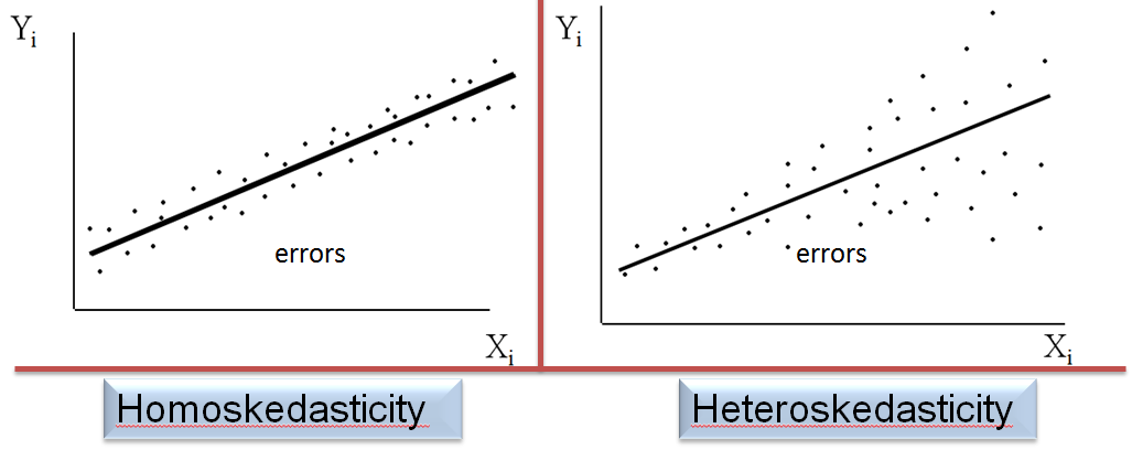
Suppose that the conditional distribution of \({ u }_{ i }\) given \({ X }_{ i }\) has a constant variance for \(i=1,\dots ,n\) which is independent of \({ X }_{ i }\). Then the error term \({ u }_{ i }\) is said to be homoskedastic otherwise it is considered heteroskedastic.
 Mathematical Implications of Homoskedasticity
The OLS estimators are unbiased and asymptotically normal – In addition to being unbiased and consistent, the estimators are furnished with normal sampling distributions in large samples. This can happen even with homoskedastic errors.
Among all linear estimators in \({ Y }_{ 1 },\dots { Y }_{ n },\) \({ \hat { \beta } }_{ 0 }\) and \({ \hat { \beta } }_{ 1 }\) are the efficient OLS estimators. The OLS estimators are also unbiased and conditional on \({ X }_{ 1 },\dots { X }_{ n }\).
A specialized formula can be applied for the standard errors of \({ \hat { \beta } }_{ 0 }\) and \({ \hat { \beta } }_{ 1 }\), in case the errors are homoskedastic. \({ \hat { \beta } }_{ 1 }\) has a homoskedasticity-only standard error of:
$$ SE\left( { \hat { \beta } }_{ 1 } \right) =\sqrt { { \hat { \sigma } }_{ { \hat { \beta } }_{ 1 } }^{ 2 } } $$
The variance of \({ \hat { \beta } }_{ 1 } \) has a homoskedasticity-only estimator that is: \({ \hat { \sigma } }_{ { \hat { \beta } }_{ 1 } }^{ 2 }\)
$$ { \hat { \sigma } }_{ { \hat { \beta } }_{ 1 } }^{ 2 }=\frac { { s }_{ \hat { u } }^{ 2 } }{ { \Sigma }_{ i=1 }^{ n }{ \left( { X }_{ i }-\bar { X } \right) }^{ 2 } } $$
The variance of all conditional estimators considered as linear functions of \({ Y }_{ 1 },\dots ,{ Y }_{ n }\) is smallest for the OLS estimator, in the event that least squares assumptions hold with errors being homoskedastic.
The OLS estimator is considered to be the Best conditionally Linear Unbiased Estimator, BLUE.
The following is the formula of the linear estimator \({ \tilde { \beta } }_{ 1 }\):
$$ { \tilde { \beta } }_{ 1 }=\sum _{ i=1 }^{ n }{ { a }_{ i }{ Y }_{ i } } $$
Rather than depending on \({ Y }_{ 1 },\dots ,{ Y }_{ n }\), the weights \({ a }_{ 1 },\dots ,{ a }_{ n }\) will depend on \({ X }_{ 1 },\dots ,{ X }_{ n }\). If the mean of the estimator \({ \tilde { \beta } }_{ 1 }\)’s conditional sampling distribution, given \({ X }_{ 1 },\dots ,{ X }_{ n }\) is \({ \beta }_{ 1 }\), then \({ \tilde { \beta } }_{ 1 }\) is conditionally unbiased. This can be written as:
$$ E\left( { \tilde { \beta } }_{ 1 }|{ X }_{ 1 },\dots ,{ X }_{ n } \right) ={ \tilde { \beta } }_{ 1 } $$
According to this theorem, the conditional variance of the OLS estimator \({ \tilde { \beta } }_{ 1 }\) is the smallest, given \({ X }_{ 1 },\dots ,{ X }_{ n }\) of all conditional estimator of \({ \beta }_{ 1 }\). This is only possible if the Gauss-Markov conditions are fulfilled. Therefore, we can say that the OLS estimator is BLUE.
These are estimators that are considered more efficient than the OLS, under some circumstances:
This is the weighted least squares method, the inverse of the square root of the conditional variance \({ u }_{ i }\) given \({ X }_{ i }\) weights the \(i\)th observation.
$$ \sum _{ j=1 }^{ n }{ |{ Y }_{ i }-{ b }_{ 0 }- } { b }_{ 1 }{ X }_{ i }| $$
The OLS estimator is said to be normally distributed, with the homoskedasticity-only \(t\)-statistic having a student’s \(t\) distribution if the following conditions referred to as the homoskedastic normal regression assumptions are fulfilled:
The distribution of \({ Z }/{ \sqrt { { W }/{ m } } }\) defines the student \(t\) distribution having \(m\) degrees of freedom. \(Z\) is a normally distributed random variable that is standard. \(W\) is a chi-squared distributed random variable having \(m\) degrees of freedom and there is no interdependence between \(Z\) and \(W\).
We can write the \(t\)-statistic calculated while applying the homoskedasticity only standard error, under the null hypothesis, in this form.
\(t={ \left( { \hat { \beta } }_{ 1 }-{ \beta }_{ 1,0 } \right) }/{ { \hat { \sigma } }_{ { \hat { \beta } }_{ 1 } }^{ 2 } }\) is the homoskedasticity-only \(t\)-statistic testing \({ \beta }_{ 1 }={ \beta }_{ 1,0 }\). \(Y\) is normally distributed conditional on \({ X }_{ 1 },\dots ,{ X }_{ n }\). Furthermore, under the null hypothesis, the distribution of \(\left( { \hat { \beta } }_{ 1 }-{ \beta }_{ 1,0 } \right)\) is normal, conditional on \({ X }_{ 1 },\dots ,{ X }_{ n }\).
Question
A trader develops a simple linear regression model to predict the price of a stock. The estimated slope coefficient for the regression is 0.60, the standard error is equal to 0.25, and the sample has 30 observations. Determine if the estimated slope coefficient is significantly different than zero at a 5% level of significance by correctly stating the decision rule.
The correct answer is B.
Step 1: State the hypothesis
H0:β1=0
H1:β1≠0
Step 2: Compute the test statistic
$$ \frac { β_1 – β_{H0} } { S_{β1} } $$
$$ \frac { 0.60 – 0} { 0.25 } = 2.4 $$
Step 3: Find critical value, t_c
From the t table, we can find t0.025,28 as 2.048
Step 4: State the decision rule
Reject H0; The slope coefficient is statistically significant since 2.048 < 2.4.
Offered by AnalystPrep


Get Ahead on Your Study Prep This Cyber Monday! Save 35% on all CFA® and FRM® Unlimited Packages. Use code CYBERMONDAY at checkout. Offer ends Dec 1st.