Correlations and Copulas

After completing this reading you should be able to:

• Define correlation and covariance and differentiate between correlation and dependence.
• Calculate covariance using the EWMA and GARCH(1,1) models.
• Apply the consistency condition to covariance.
• Describe the procedure of generating samples from a bivariate normal distribution.
• Describe properties of correlations between normally distributed variables when using a one-factor model.
• Define copula and describe the key properties of copulas and copula correlation.
• Explain tail dependence.
• Describe Gaussian copula, Student’s t-copula, multivariate copula, and one-factor copula.

Correlation

Assuming that we have two variables namely \({ V }_{ 1 }\) and \({ V }_{ 2 }\), then the correlation coefficient denoted as \(\rho\) is:

$$ \rho =\frac { E\left( { V }_{ 1 }{ V }_{ 2 } \right) -E\left( { V }_{ 1 } \right) E\left( { V }_{ 2 } \right) }{ SD\left( { V }_{ 1 } \right) SD\left( { V }_{ 2 } \right) } $$

\(SD\) is the standard deviation and \(E\left( . \right) \) is the expected value. Absent correlation we have that:

$$ E\left( { V }_{ 1 }{ V }_{ 2 } \right) =E\left( { V }_{ 1 } \right) E\left( { V }_{ 2 } \right) $$

$$ \Rightarrow \rho =0 $$

If \({ V }_{ 1 }={ V }_{ 2 }\) then \(\rho=1\) since the variance of \({ V }_{ 1 }\) will be equal to both the numerator and the denominator in the equation for \(\rho\).

Correlation vs Dependence

For \({ V }_{ 1 }\) and \({ V }_{ 2 }\) to be independent, then:

$$ f\left( { V }_{ 2 }|{ V }_{ 1 }=x \right) =f\left( { V }_{ 2 } \right) \quad for\quad all\quad x. $$

The \(PDF\) is denoted by \(f\left( . \right) \), and the conditional one-factor is denoted as \(|\).

A correlation coefficient of zero between two variables does not necessarily imply lack of dependence between the two variables. The correlation coefficient is a measure of a single form of dependence between the variables, with the dependence being linear.

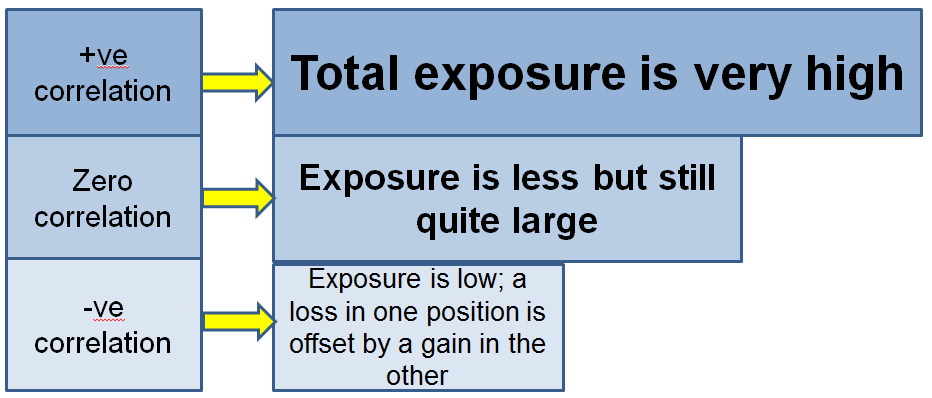
But why is it important to estimate the degree of co-movement between two assets? Suppose that a company has an exposure to two different positions. Each position gains $100 million if there is a one-standard-deviation increase and loses $100 million if there is a one-standard-deviation decrease. Therefore, we can sum it up in the following graph:

Should we evaluate the standard deviation of \({ V }_{ 2 }\) conditional on \({ V }_{ 1 }\), will simply be looking at the dependence of \({ V }_{ 2 }\) on \({ V }_{ 1 }\), only from a different angle.

Monitoring Correlation

Let variables \(X\) and \(Y\) have values \({ X }_{ i }\) and \({ Y }_{ i }\) at the closure of day \(i\). On day \(i\), the variables will have the following returns:

$$ { x }_{ i }=\frac { { X }_{ i }-{ X }_{ i-1 } }{ { X }_{ i-1 } } $$

And:

$$ { y }_{ i }=\frac { { Y }_{ i }-{ Y }_{ i-1 } }{ { Y }_{ i-1 } } $$

On day \(n\) we will have the following covariance rate between \(X\) and \(Y\):

$$ { cov }_{ n }=E\left( { x }_{ n }{ y }_{ n } \right) -E\left( { x }_{ n } \right) E\left( { y }_{ n } \right) $$

Suppose that on computing the variance rate per day the expected daily returns are zero, then on day \(n\) the following equation represents the covariance rate per day between \(X\) and \(Y\):

$$ { cov }_{ n }=E\left( { x }_{ n }{ y }_{ n } \right) $$

When equal weights for the last \(m\) observations are applied on \({ x }_{ i }\) and \({ y }_{ i }\), then we hace:

$$ { cov }_{ n }=\frac { 1 }{ m } \sum _{ i=1 }^{ m }{ { x }_{ n-i }{ y }_{ n-i } } $$

On day \(n\), variable \(X\) will have the following variance rate:

$$ { var }_{ x,n }=\frac { 1 }{ m } \sum _{ i=1 }^{ m }{ { x }_{ n-1 }^{ 2 } } $$

And the variance rate for variable \(Y\) is:

$$ { var }_{ y,n }=\frac { 1 }{ m } \sum _{ i=1 }^{ m }{ { y }_{ n-1 }^{ 2 } } $$

On day \(n\), the correlation is estimated as:

$$ \frac { { cov }_{ n } }{ \sqrt { { var }_{ x,n }{ var }_{ y,n } } } $$

EWMA

In this model, a covariance estimate can be updated by the following formula:

$$ { cov }_{ n }=\lambda { cov }_{ n-1 }+\left( 1-\lambda \right) { x }_{ n-i }{ y }_{ n-i } $$

As \(i\) increases, the weights accorded to \({ x }_{ n-i }{ y }_{ n-i }\) falls. A lower \(\lambda\) implies that the recent observations have been accorded a greater weight.

GARCH

With GARCH models, estimates of covariance rate can be updated and the future level of covariance rates be forecasted. A covariance between \(X\) and \(Y\) can be updated using the following GARCH (1, 1) model:

$$ { cov }_{ n }=\omega +\alpha { x }_{ n-1 }{ y }_{ n-1 }+\beta { cov }_{ n-1 } $$

The long-term average covariance rate is expressed as:

$$ \frac { \omega }{ 1-\alpha -\beta } $$

Consistency Condition for Covariances

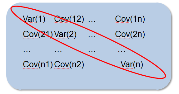
We can create a variance-covariance matrix after computing the variance rate and covariance rate for a set of market variables. Between variable \(i\) and variable \(j\), the covariance rate is depicted by the \(\left( i,j \right) \) element of the matrix, with \(i\neq j\). Variable \(i\)’s variance rate is depicted when \(i= j\).

The \(N \times N\) variance-covariance matrix is denoted by \(\Omega \), and for it to be internally consistent, then:

$$ { w }^{ T }\Omega w\ge 0 $$

This is true for all \(N \times 1\) vectors \(w\), with \({ w }^{ T }\) being the transpose of \(w\). This property is satisfied by a matrix called positive-semidefinite. Assuming that we have a column vector \(w:\left( { w }_{ 1 },{ w }_{ 2 },\dots ,{ w }_{ N } \right) \), if an investment of amount \({ w }_{ i }\) is injected in the market variable \(i\), then the portfolio will have a non-negative variance rate denoted as \({ w }^{ T }\Omega w\).

Multivariate Normal Distributions

Let’s assume that we have a bivariate normal distribution whose only variables are \({ V }_{ 1 }\) and \({ V }_{ 2 }\). Assuming also we are aware of the value of \({ V }_{ 1 }\). Therefore, the value of \({ V }_{ 2 }\) conditional on this is normal with a mean of:

$$ { \mu }_{ 2 }+\rho { \sigma }_{ 2 }\frac { { V }_{ 1 }-{ \mu }_{ 1 } }{ { \sigma }_{ 1 } } $$

And with a standard deviation of:

$$ { \sigma }_{ 2 }\sqrt { 1-{ \rho }^{ 2 } } $$

The unconditional means of \({ V }_{ 1 }\) and \({ V }_{ 2 }\) are denoted as \({ \mu }_{ 1 }\) and \({ \mu }_{ 2 }\) respectively. The unconditional standard deviations of \({ V }_{ 1 }\) and \({ V }_{ 2 }\) are \({ \sigma }_{ 1 }\) and \({ \sigma }_{ 2 }\) respectively. The correlation coefficient between \({ V }_{ 1 }\) and \({ V }_{ 2 }\) is denoted as \(\rho\). Furthermore, the reader should take note that there is a linear dependence on the value of \({ V }_{ 1 }\) by the expected value of \({ V }_{ 2 }\) conditional on \({ V }_{ 1 }\).

Generating Random Samples from Normal Distributions

Suppose samples \({ \epsilon }_{ 1 }\) and \({ \epsilon }_{ 2 }\) are to be drawn from a bivariate normal distribution as a requirement. The mean and standard deviation of both variables are 0 and 1 respectively. The independent samples \({ z }_{ 1 }\) and \({ z }_{ 2 }\) are first determined from a univariate standardized normal distribution. We then compute the required samples \({ \epsilon }_{ 1 }\) and \({ \epsilon }_{ 2 }\) in the following manner:

$$ { \epsilon }_{ 1 }={ z }_{ 1 } $$

$$ { \epsilon }_{ 1 }=\rho { z }_{ 1 }+{ z }_{ 2 }\sqrt { 1-{ \rho }^{ 2 } } $$

With the bivariate normal distribution having a correlation coefficient denoted as \(\rho\).

Let us now assume that we are in a position whereby the required samples should be from a multivariate normal distribution and the mean and standard deviation of all the variables are 0 and 1 respectively. Moreover, \({ \rho }_{ ij }\) is to considered as the correlation coefficient between variables \(i\) and \(j\). To begin with, \(n\) independent variables \({ z }_{ i }\left( 1\le i\le n \right) \) are sampled from univariate standardized normal distributions.

The following is an expression for the required samples:

$$ { \epsilon }_{ i }\left( 1\le i\le n \right) $$

And:

$$ { \epsilon }_{ i }=\sum _{ k=1 }^{ i }{ { \alpha }_{ ik }{ z }_{ k } } $$

There are \({ \alpha }_{ ik }\) parameters considered for the accurate variances and correlations for the \({ \epsilon }_{ i }\). If \( 1\le j\le i \), then:

$$ { \Sigma }_{ k=1 }^{ i }{ \alpha }_{ ik }^{ 2 }=1 $$

For all \(j < 1\), then:

$$ \sum _{ k=1 }^{ j }{ { \alpha }_{ ik }{ \alpha }_{ jk } } ={ \rho }_{ ij } $$

Since \({ \epsilon }_{ 1 }={ z }_{ 1 }\), then we can compute \({ \epsilon }_{ 2 }\) from \({ z }_{ 1 }\) and \({ z }_{ 2 }\) and \({ \epsilon }_{ 3 }\) from \({ z }_{ 1 },{ z }_{ 2 }\),and \({ z }_{ 3 }\). We can continue in this manner under a procedure referred to as the Cholesky decomposition.

Factor Models

A factor model can be applied in the definition of the correlations between normally distributed variables. Let us consider \({ U }_{ 1 },{ U }_{ 2 },\dots ,{ U }_{ N }\) having standard normal distributions. The component of each \({ U }_{ i }\) is dependent on a common factor, \(F\), and uncorrelated with the other variables, in a model that is one-factor. Therefore:

$$ { U }_{ i }={ a }_{ i }F+\sqrt { 1-{ a }_{ i }^{ 2 } } { Z }_{ i } $$

The standard normal distributions are denoted as \(F\) and \({ Z }_{ i }\). The constant between -1 and +1 is \({ a }_{ j }\). Furthermore, the \({ Z }_{ i }\) are uncorrelated with one another and with \(F\). We select the coefficient of \({ Z }_{ i }\) in a manner that the mean an variance of \({ U }_{ j }\) will be 0 and 1 respectively. Between \({ U }_{ i }\) and \({ U }_{ j }\), the correlation coefficient is \({ a }_{ i } { a }_{ j }\).

Absent the assumption of a factor model, we will have to estimate \({ N\left( N-1 \right) }/{ 2 }\) correlations for \(N\) variables. On the other hand, only \(N\) parameters namely \({ a }_{ 1 },{ a }_{ 2 },\dots ,{ a }_{ N }\) need to be estimated, with the one-factor model.

The concept of a one-factor model can be generally modified to an \(M\)-factor model, such that:

$$ { U }_{ i }={ a }_{ i1 }{ F }_{ 1 }+{ a }_{ i2 }{ F }_{ 2 }+\cdots +{ a }_{ iM }{ F }_{ M }+\sqrt { 1-{ a }_{ i1 }^{ 2 }-{ a }_{ i2 }^{ 2 }-\cdots -{ a }_{ iM }^{ 2 } } { Z }_{ i } $$

In the above equation, the \({ F }_{ i }\)’s have standard normal distributions that are uncorrelated. For \({ Z }_{ i }\) the correlation is both with each other and with the factors. Therefore, the following is the expression for the correlation between \({ U }_{ i }\) and \({ U }_{ j }\):

$$ { \Sigma }_{ m=1 }^{ M }{ a }_{ im }{ a }_{ jm } $$

Copulas

Let \({ V }_{ 1 }\) and \({ V }_{ 2 }\) be two variables that are correlated. If we have no information on \({ V }_{ 2 }\) then \({ V }_{ 1 }\) has a distribution that is called marginal or unconditional distribution. The opposite is also true for \({ V }_{ 2 }\). supposing that the marginal distributions of \({ V }_{ 1 }\) and \({ V }_{ 2 }\) are estimated. In case \({ V }_{ 1 }\) and \({ V }_{ 2 }\) have normal marginal distributions, then the assumption that we have a bivariate normal joint distribution of the variables is the best and most convenient to use.

Copulas are applicable in situations where a correlation structure between two marginal distributions lacks a natural definition. In this regard, consider two variables \({ V }_{ 1 }\) and \({ V }_{ 2 }\) with triangular PDFs and whose values range from 0 to 1. \({ V }_{ 1 }\) and \({ V }_{ 2 }\) can be mapped into two variables \({ U }_{ 1 }\) and \({ U }_{ 2 }\) whose distributions are standard normal, using a Gaussian Copula on the basis of percentile-to-percentile.

\({ U }_{ 1 }\) and \({ U }_{ 2 }\) are normally distributed variables and are considered as jointly bivariate normal. A joint distribution together with a correlation structure between \({ V }_{ 1 }\) and \({ V }_{ 2 }\) is the implication. The copula is therefore applicable in the sense that correlation structure is defined indirectly rather than directly between \({ V }_{ 1 }\) and \({ V }_{ 2 }\).

This implies that \({ V }_{ 1 }\) and \({ V }_{ 2 }\) are mapped into other variables where correlation structure can be easily defined. Between \({ U }_{ 1 }\) and \({ U }_{ 2 }\) the correlation is called copula correlation.

Algebraic Expression to the Approach

Let the cumulative marginal probability distribution of \({ V }_{ 1 }\) and \({ V }_{ 2 }\) be \({ G }_{ 1 }\) and \({ G }_{ 2 }\). We map, \({ V }_{ 1 }={ v }_{ 1 }\),\({ U }_{ 1 }={ u }_{ 1 }\) and \({ V }_{ 2 }={ v }_{ 2 }\),\({ U }_{ 2 }={ u }_{ 2 }\).

Therefore:

$$ { G }_{ 1 }\left( { V }_{ 1 } \right) =N\left( { U }_{ 1 } \right) $$

And:

$$ { G }_{ 2 }\left( { V }_{ 2 } \right) =N\left( { U }_{ 2 } \right) $$

The cumulative normal distribution of the function is denoted as \(N\). This implies that:

$$ u_{ 1 }={ N }^{ -1 }\left[ { G }_{ 1 }\left( { V }_{ 1 } \right) \right] $$

$$ u_{ 2 }={ N }^{ -1 }\left[ { G }_{ 2 }\left( { V }_{ 2 } \right) \right] $$

And:

$$ v_{ 1 }={ G }_{ 1 }^{ -1 }\left[ N\left( { u }_{ 1 } \right) \right] $$

$$ v_{ 2 }={ G }_{ 2 }^{ -1 }\left[ N\left( { u }_{ 2 } \right) \right] $$

Therefore, \({ U }_{ 1 }\) and \({ U }_{ 2 }\) are considered bivariate normal variables.

Tail Dependence

Tail dependence is the tendency for extreme values for two variables to occur together. It usually occurs when the correlation between two variables increases as you get “further” in the tail (either or both) of the distribution.

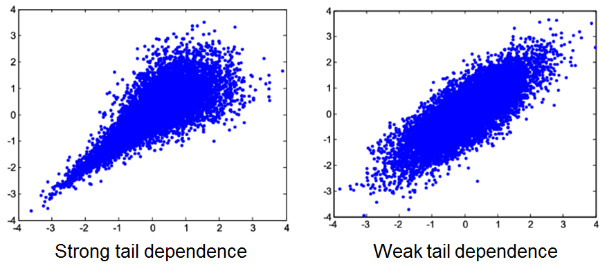
Financial markets tend to exhibit tail-dependence, especially lower tail dependence. For instance, major stock returns in stable economic conditions have a correlation of, roughly 0.5. In the height of the 2007/2008 financial crisis, however, some pairs had correlations as high as 0.9 – indicating a high possibility of “dual” failure.

Default risk models used at the time did not take into account tail dependence. As a result, the models under-estimated potential losses. After the housing burble burst, the correlation of homeowners’ payments (random variables) significantly increased.

Multivariate Copulas

In cases where there more than two variables, the correlation structure between them can be defined with copulas. The multivariate Gaussian copula is an example of a multivariate copula. Consider the following \(N\) variables where the marginal distribution of each is known \({ V }_{ 1 },{ V }_{ 2 },\dots ,{ V }_{ N }\). \({ V }_{ i }\) can be mapped into \({ U }_{ i }\), for each \(i\left( 1\le i\le N \right) \), with the distribution of \({ U }_{ i }\) being standard normal. \({ U }_{ i }\) is therefore considered as having a multivariate normal distribution.

A Factor Copula Model

A factor model for the correlation structure between \({ U }_{ i }\) is a common assumption in multivariate copula models. When only one factor exists, then:

$$ { U }_{ i }={ a }_{ i }F+\sqrt { 1-{ a }_{ i }^{ 2 }{ Z }_{ i } } \quad \quad \quad equation\quad I $$

In the above equation, the standard normal distributions are \(F\) and \({ Z }_{ i }\). There is uncorrelation between the \({ Z }_{ i }\)’s themselves and between them with \(F\).

Application to Loan Portfolios: Vasicek’s Model

We wish to model a portfolio’s loan defaults. Let company \(i\) default at a time \({ T }_{ i }\). All loans are assumed to be having a similar cumulative probability distribution for the default time. Let PD be the likelihood of default by the time \(T\).

Such that:

$$ PD=Prob\left( { T }_{ i }<T \right) $$

We can apply the Gaussian Copula Model in defining the correlation structure between the loans’ time to default.

Let’s assume that the \({ a }_{ i }\) are similar and equivalent to \(a\). Therefore:

$$ { U }_{ i }=aF+\sqrt { 1-{ a }^{ 2 }{ Z }_{ i } } $$

The assumption here is the factor model in the equation \(I\) for the correlation structure between the \({ U }_{ i }\). In this case pair of loans has the same copula correlation between them, given as:

$$ \rho ={ a }^{ 2 } $$

\({ U }_{ i }\) can therefore be expressed as follows:

$$ { U }_{ i }=\sqrt { \rho } F+\sqrt { 1-\rho } { Z }_{ i }\quad \quad \quad equation\quad II $$

The worst case default rate \(WCDR\) (\(T, X\)) is the default rate during time \(T\) that will not be surpassed with probability \(X\)%.

Therefore:

$$ WCDR\left( T,X \right) =N\left( \frac { { N }^{ -1 }PD-\sqrt { \rho } { N }^{ -1 }\left( X \right) }{ \sqrt { 1-\rho } } \right) $$

Proof of Vasicek’s Result

The following relation is based on the properties of the Gaussian Copula Model:

$$ PD=Prob\left( { T }_{ i }<T \right) =Prob\left( { U }_{ i }<U \right) $$

And:

$$ U={ N }^{ -1 }\left[ PD \right] $$

The value of factor, \(F\) in equation \(II\) above affects the default likelihood by time \(T\). Consider the default likelihood conditional on \(F\).

From equation \(II\), we can deduce that:

$$ { Z }_{ i }=\frac { { U }_{ i }-\sqrt { \rho } F }{ \sqrt { 1-\rho } } $$

Conditional on the factor value,\( F\), the likelihood that \({ U }_{ i }<U\) can be expressed as:

$$ Prob\left( { U }_{ i }<U|F \right) =Prob\left( { Z }_{ i }<\frac { { U }-\sqrt { \rho } F }{ \sqrt { 1-\rho } } \right) =N\left( \frac { { U }-\sqrt { \rho } F }{ \sqrt { 1-\rho } } \right) $$

Thus:

$$ Prob\left( { T }_{ i }<T|F \right) =N\left( \frac { { U }-\sqrt { \rho } F }{ \sqrt { 1-\rho } } \right) $$

This implies that:

$$ Prob\left( { T }_{ i }<T|F \right) =N\left( \frac { { { N }^{ -1 }\left( PD \right) }-\sqrt { \rho } F }{ \sqrt { 1-\rho } } \right) $$

An increase in \(F\) causes a corresponding increase in the rate of default. The probability of \(F\) being less than \({ { N }^{ -1 }\left( Y \right) }\) is \(Y\), (due to the fact that \(F\) is normally distributed). This implies that \(Y\) is the likelihood the rate of default will surpass:

$$ N\left( \frac { { { N }^{ -1 }\left( PD \right) }-\sqrt { \rho } { N }^{ -1 }\left( Y \right) }{ \sqrt { 1-\rho } } \right) $$

Estimating PD and ρ

Let \(DR\) denote the rate of default. The cumulative \(PDF\) for \(DR\) will be denoted as \(G\left( D,R \right) \). Then we have that:

$$ DR=N\left( \frac { { { N }^{ -1 }\left( PD \right) }+\sqrt { \rho } { N }^{ -1 }\left( G\left( DR \right) \right) }{ \sqrt { 1-\rho } } \right) $$

Hence:

$$ G\left( DR \right) =N\left( \frac { { { \sqrt { 1-\rho } N }^{ -1 }\left( DR \right) }-{ N }^{ -1 }\left( PD \right) }{ \sqrt { \rho } } \right) \quad \quad \quad IIA $$

Differentiating this, the default rate has the following \(PDF\):

$$ G\left( DR \right) =\sqrt { \frac { 1-\rho }{ \rho } } exp\left\{ \frac { 1 }{ 2 } \left[ { \left( { N }^{ -1 }\left( DR \right) \right) }^{ 2 }-{ \left( \frac { { { \sqrt { 1-\rho } N }^{ -1 }\left( DR \right) }-{ N }^{ -1 }\left( PD \right) }{ \sqrt { \rho } } \right) }^{ 2 } \right] \right\} \quad \quad \quad \quad \quad III $$

We can always apply the following procedure to compute the estimates of maximum probability for \(PD\) and \(\rho\) from historical data:

1. Trial values of \(PD\) and \(\rho\) should be chosen,
2. The logarithm of the probability density in equation \(III\) above should be computed for each of the observations on \(DR\).
3. The values of \(PD\) and \(\rho\) maximizing the sum of values in procedure (\(b\)) above should be searched using Solver.

Alternatives to the Gaussian Copula

Other one-factor copulas are developed by choosing \(F\) or \({ Z }_{ i }\), or both, as distributions having heavier tails as compared to the normal distribution in equation \(II\). The distributions of \(F\) and \({ Z }_{ i }\) are applied to determine the distribution of \({ U }_{ i }\).

Therefore:

$$ WCDR\left( T,X \right) =\Phi \left( \frac { { \Psi }^{ -1 }PD-\sqrt { \rho } { \Theta }^{ -1 }\left( X \right) }{ \sqrt { 1-\rho } } \right) $$

The cumulative probability distributions of \(F\),\({ Z }_{ i }\), and \({ U }_{ i }\) are denoted as \(\Theta \),\(\Phi \),and \(\Psi \). Equation \(IIA\) changes to:

$$ G\left( DR \right) =\Phi { \left( \frac { { { \sqrt { 1-\rho } \Phi }^{ -1 }\left( DR \right) }-{ \Psi }^{ -1 }\left( PD \right) }{ \sqrt { \rho } } \right) } $$

Question 1

An analyst uses the EWMA model with λ = 0.92 to update correlation and covariance rates.The correlation estimate for two variables A and B on day n − 1 is 0.7. The estimated standard deviations on day n − 1 for variables A and B are 2% and 2.5%, respectively. Also, the percentage change on day n − 1 for variables A and B are 3% and 2%, respectively.

What is the updated estimate of the covariance rate between A and B on day n?

1. 0.0035
2. 0.0037
3. 0.00035
4. 0.00037

The correct answer is D.

The estimated covariance rate between variables X and Y on day n − 1 can be calculated as:

$$ { cov }_{ n }=\rho_{ A,B }×\sigma_{ A }\sigma_{ B } =0.7×0.02×0.025=0.00035 $$

With the latest covariance rate, the EWMA model can update the covariance rate for day n:

$$ { cov }_{ n }=\lambda { cov }_{ n-1 }+\left( 1-\lambda \right) { x }_{ n-i }{ y }_{ n-i } = 0.92×0.00035+0.08×0.03×0.02 = 0.00037$$