Simulation and Bootstrapping

After completing this reading, you should be able to:

• Describe the basic steps to conduct a Monte Carlo simulation.
• Describe ways to reduce the Monte Carlo sampling error.
• Explain the use of antithetic and control variates in reducing Monte Carlo sampling error.
• Describe the bootstrapping method and its advantage over the Monte Carlo simulation.
• Describe pseudo-random number generation.
• Describe situations where the bootstrapping method is ineffective.
• Describe the disadvantages of the simulation approach to financial problem-solving.

Introduction and Definitions

Simulation is a way of modeling random events to match real-world outcomes. By observing simulated results, researchers gain insight into real problems. Examples of the application of the simulation are the calculation of option payoff and determining the accuracy of an estimator. Some of the simulation methods are the Monte Carlo Simulation (Monte Carlo) and the Bootstrapping.

Monte Carlo Simulation approximates the expected value of a random variable using the numerical methods. The Monte Carlo generates the random variables from an assumed data generating process (DGP), and then it applies a function(s) to create realizations from the unknown distribution of the transformed random variables. This process is repeated (to improve the accuracy), and the statistic of interest is then approximated using the simulated values.

Bootstrapping is a type of simulation where it uses the observed variables to simulate from the unknown distribution that generates the observed variables. In other words, bootstrapping involves the combination of the observed data and the simulated values to create a new sample that is related but different from the observed data.

The notable similarity between Monte Carlo and bootstrapping is that both aim at calculating the expected value of the function by using simulated data (often by use of a computer).

Also, the contrasting feature in these methods is that in Monte Carlo simulation, a data generating process (DGP) is entirely used to simulate the data. However, in bootstrapping, observed data is used to generate the simulated data without specifying an underlying DGP.

Simulation of Random Variables

The simulation requires the generation of random variables from an assumed distribution, mostly using a computer. However, computer-generated numbers are not necessarily random and thus termed as pseudo-random numbers. Pseudo numbers are produced by the complex deterministic functions (pseudo number generators, PNGs), which seem to be random. The initial values of pseudo numbers are termed as a seed value, which is usually unique but generates similar random variables when PNRG runs.

The ability of the simulated variables from PRNGs to replicate makes it possible to use pseudo numbers across multiple experiments because the same sequence of random variables can be generated using the same seed value. Therefore, we can use this feature to choose the best model or reproduce the same results in the future in case of regulatory requirements. Moreover, the corresponding random variables can be generated using different computers.

Simulating Random Variables from a Specific Distribution

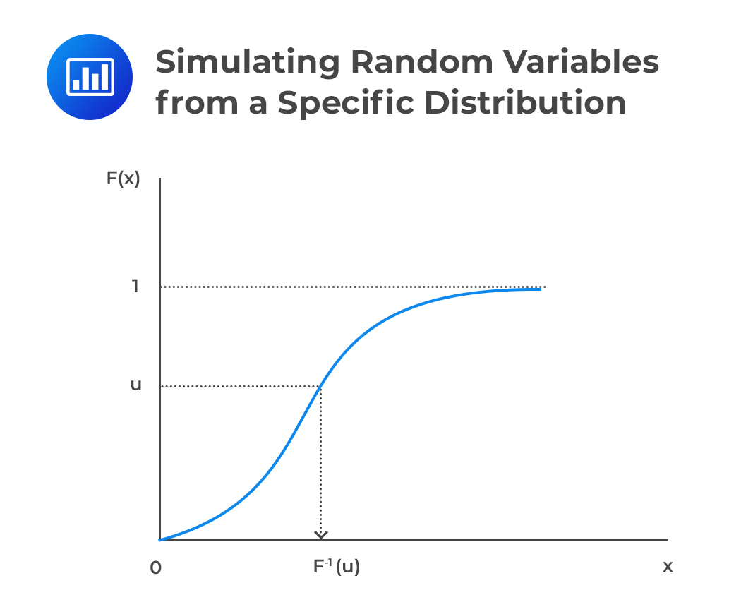
Simulating random variables from a specific distribution is initiated by first generating a random number from a uniform distribution (0,1). After that, the cumulative distribution of the distribution we are trying to simulate is used to get the random values from that distribution. That is, we first generate a random number U from U(0,1) distribution, then, we use the generated random number to simulate a random variable X with the pdf f(x) by using the CDF, F(x).

Let U be the probability that X takes a value less than or equal to x, that is,

$$ \text U=\text P( \le \text x)=\text F(\text x) $$

Then we can derive the random variable x as:

$$ \text x=\text F^{-1} (\text u) $$

To put this in a more straightforward perspective, the algorithm for simulating random variable from a specific distribution involves:

1. Generating a random variable u from the uniform distribution U(0,1)
2. Compute \(\text x=\text F^{-1} (\text u)\)

Note that the random variable X has a CDF F(x) as shown below:

$$ \text P(\text X \le {\text x})=\text P(\text F^{-1} (\text U) \le {\text x})=\text P(\text U \le {\text F}(\text x))=\text F(\text x) $$

Example: Generating Random Variables from Exponential Distribution

Assume that we want to simulate three random variables from an exponential distribution with a parameter \(\lambda=0.2\) using the value 0.112, 0.508, and 0.005 from U(0,1).

Solution

This question assumes that the uniform random variable has been generated. The inverse of the CDF of exponential distribution is given by:

$$ \text F^{-1} (\text x)=-\frac {1}{\lambda} \text{ln⁡ }(1-\text x) $$

So, in this case:

$$ \begin{align*} \text F^{-1} (\text x) & =-\cfrac {1}{0.2} \text{ln }⁡(1-\text x) \\ \text x & =-\cfrac {1}{0.2} \text{ln }⁡(1-\text u) \\ \end{align*} $$

So the random variables are:

$$ \begin{align*} {\text x}_1 & =-\cfrac {1}{0.2} \text{ln }(1-{\text u}_1 )=-5\text{ ln⁡ }(1-0.112)=2.37567 \\ {\text x}_2 & =-\cfrac {1}{0.2} \text{ln }(1-{\text u}_2 )=-5 \text{ ln⁡ }(1-0.508)=14.1855 \\ {\text x}_3 & =-\cfrac {1}{0.2} \text{ln }(1-{\text u}_3 )=-5\text{ ln⁡ }(1-0.005)=0.10025 \\ \end{align*} $$

The random variables are 2.37567, 14.1855 and 0.10025

Monte Carlo Simulation

Monte Carlo simulation is used to estimate the population moments or functions. The Monte Carlo is as follows:

Assume that X is a random variable that can be simulated and let g(X) be a function that can be evaluated at the realizations of X. Then, the simulation generates multiple copies of g(X) by simulating draws from \(\text X=\text x_{\text j}\) and calculate \(\text g_{\text i}=\text g(\text x_{\text i})\).

This process is then repeated b times so that a set of iid variables is generated from the unknown distribution g(X), which can then be used to estimate the desired statistic.

For instance, if we wish to estimate the mean of the generated random variables, then the mean is given by:

$$ \hat {\text E}(\text g(\text X))=\cfrac {1}{\text b} \sum_{\text i=1}^{\text b} \text g(\text X_{\text i}) $$

This is true because the generated variables are iid, and then the process is repeated b times. Consequently, by the law of large number (LLN),

$$ \lim_{ b\rightarrow \infty }{ \hat {\text E}(\text g(\text X)) } ={\text E}(\text g(\text x)) $$

Also, the Central Limit Theorem applies to the estimated mean so that:

$$ \text{Var}[\hat {\text E}(\text g(\text X))]=\cfrac {\sigma_{\text g}^2}{\text b} $$

Where \({\sigma_{\text g}^2}=\text{Var}(\text g(\text X))\)

The second moment, which is the variance (standard variance estimator) is estimated as:

$$ {\hat \sigma_{\text g}^2}=\cfrac {1}{\text b} \sum_{\text i=1}^{\text b} \left(\text g(\text X_{\text i} )-\text E[\widehat { g(X)}] \right)^2 $$

From CLT, the standard error of the simulated expectation is given by:

$$ \sqrt{\cfrac {{ \sigma_{\text g}^2}}{\text b}}=\cfrac {\sigma_2}{\sqrt {\text b}} $$

The standard error of the simulated expectation measures the level of accuracy of the estimation; thus, the choice of b determines the accuracy of the simulation.,

Another quantity that can be calculated from the simulation is the \(\bf {\alpha}\)-quantile by arranging the b draws in ascending order then selecting the value \(\bf{b{\alpha}}\) of the sorted set.

Moreover, using the simulation, we determine the finite sample properties of the estimated parameters. Assume that the sample size n is large enough so that approximation by CLT is adequate. Now, consider a finite-sample distribution of a parameter \(\hat \theta\). Using the assumed DGP, n random samples are generated so that:

$$ \text X=[\text x_1,\text x_2,…,\text x_{\text n} ] $$

We need to estimate a parameter \(\hat \theta\).

We would need to simulate new data set and estimate the parameter b times: \((\hat \theta_1,\hat \theta_2,…,\hat \theta_{\text b})\) from the finite-sample distribution of the estimator of \(\theta\). From these values, we can rule out the properties of the estimator \(\hat \theta\). For instance, the bias defined as:

$$ \text{Bias}(\theta)=\text E(\hat \theta)-\theta $$

That can be approximated as:

$$ {\widehat {(\text{Bias})}}(\theta)=\cfrac {1}{\text b} \sum_{\text i=1}^{\text b}(\hat \theta_{\text i}-\theta) $$

Having the basics of the Monte Carlo simulation, its basic logarithm is as follows:

1. Generate the data: \(\text x_i=[\text x_{1\text i},\text x_{2\text i},…,\text x_{\text {ni}}]\) by using the assumed DGP.
2. Compute the desired function or statistic \(\text g_{\text i}=\text g(\text x_{\text i} )\).
3. Iterate steps 1 and 2 b times.
4. From the replications \(\left\{\text g_1,\text g_2,…,\text g_{\text b}\right\}\), calculate the statistic of interest.
5. Determine the accuracy of the estimated quantity by calculating the standard error. If the standard error is huge, increase the number of b-replications to obtain the smallest error possible.

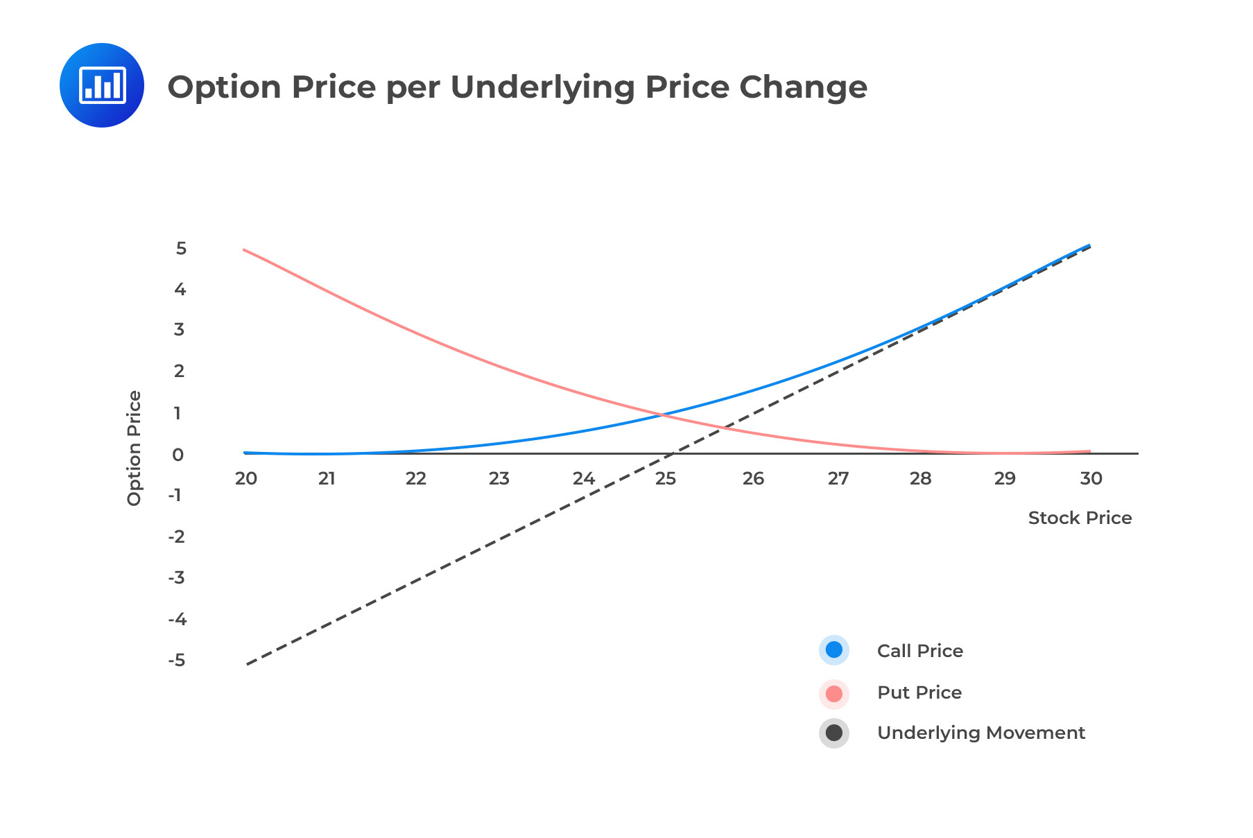
Example: Using the Monte Carlo Simulation to Estimate the Price of a Call Option

Recall that the price of a call option is given by:

$$ \text{max}⁡(0,\text S_{\text T}-\text K) $$

\(\text S_{\text T}\) is the price of the underlying stock at the time of maturity T, and K is the strike price. The price of the call option is a non-linear function of the underlying stock price at the expiration date, and thus, we can model the price of the call option.

Assuming that the log of the stock price is normally distributed, then the price of the stock can be modeled as the sum of the initial stock price, a mean and normally distributed error. Mathematically stated as:

$$ \text s_{\text T}=\text s_0+\text T \left(\text r_{\text f}-\cfrac {\sigma^2}{2}\right) \sqrt {\text T} \text x_{\text i} $$

Where

\(\text s_0\)= the initial stock price

T= time to maturity in years

\(\text r_{\text f}\)= annualized time to maturity

\(\sigma^2\)= variance of the stock return

\(\text x_{\text i}\)= simulated values from \(\text N(0,\sigma^2)\)

From the formula above, to simulate the price of the underlying stock requires the estimation of the stock volatility.

Using the simulated price of the stock, the price of the option can be calculated as:

$$ \text c=\text e^{(-\text r_{\text f} \text T)} \text {max}(\text S_{\text T}-\text K,0) $$

And thus the mean of the price of the call option can be estimated as:

$$ \hat {\text E}(\text c)=\bar {\text c}=\cfrac {1}{\text b} \sum_{\text i=1}^{\text b} \text c_{\text i} $$

Where \(\text c_{\text i}\) is the simulated payoffs of the call option. Note that, using the equation, \(\text s_{\text T}=\text s_0+\text T \left(\text r_{\text f}-\cfrac {\sigma^2}{2}\right) \sqrt {\text T} \text x_{\text i}\), the simulated stock prices can be expressed as:

$$ \text S_{\text {Ti}}=\text e^{\text s_0+\text T \left(\text r_{\text f}-\cfrac {\sigma^2}{2} \right)+\sqrt {\text T} \text x_{\text i} } $$

And thus

$$ \text g(\text x_{\text i} )=\text c_{\text i}=\text e^{(-\text {rT})} \text {max}⁡ \left(\text e^{\text s_0+\text T(\text r_{\text f}-\frac {\sigma^2}{2})+\sqrt{\text T} \text x_{\text i} }-\text K,0 \right) $$

The standard error of the call option price is given by:

$$ \text {s.e} \left({\hat {\text E}}(\text c) \right)=\sqrt{ \cfrac {\hat \sigma_{\text g}^2}{\text b} }=\cfrac {{\hat \sigma}_{\text g}}{\sqrt{\text b}} $$

Where \({\hat \sigma_{\text g}^2}\)

$$ {\hat \sigma_{\text g}^2}=\cfrac {1}{\text b} \sum_{\forall {\text i}} (\text c_{\text i}-\hat {\text c})^2 $$

Given that we calculate the standard error, we can calculate the confidence intervals for the estimated mean of the call option price. For instance, the 95% confidence interval; is given by:

$$ \hat {\text E}(\text c) \pm 1.96 \text{ s.e } \left(\hat {\text E}(\text c) \right) $$

Reducing Monte Carlo Sampling Error

Sampling error in Monte Carlo simulation is reduced by two complementary methods:

1. Antithetic Variables, and
2. Control Variates.

These methods can be used simultaneously.

To set the mood, recall that the estimation of expected values in simulation depends on the Law of Large Numbers (LLN) and that the standard error of the estimated expected value is proportional to 1/√b. Therefore, the accuracy of the simulation depends on the variance of the simulated quantities.

Antithetic Variables

Recall variance between two random variables X and Y is given by:

$$ \text {Var}(\text X+\text Y)=\text {Var}(\text X)+\text {Var}(\text Y)+2\text {Cov}(\text X,\text Y) $$

Otherwise, if the variables are independent, then:

$$ \text {Var}(\text X+\text Y)=\text {Var}(\text X)+\text {Var}(\text Y) $$

Moreover, if the covariance between the variables is negative (or negatively correlated), then:

$$ \text {Var}(\text X+\text Y)=\text {Var}(\text X)+\text {Var}(\text Y)-2\text {Cov}(\text X,\text Y) $$

The antithetic variables use the last result. The antithetic variables reduce the sampling error by incorporating the second set of variables that are generated in such a way that they are negatively correlated with the initial iid simulated variables. That is, each simulated variable is paired with an antithetic variable so that they occur in pairs and are negatively correlated.

If \(\text U_1\) is a uniform random variable, then:

$$ \text F^{-1} (\text U_1 ) \sim \text F_{\text x} $$

Denote an antithetic variable \(\text U_2\) which is generated using:

$$ \text U_2=1-\text U_1 $$

Note that \(\text U_2\) is also a uniform random variable so that:

$$ \text F^{-1} (\text U_2 )\sim \text F_{\text x} $$

Then by definition of antithetic variables, the correlation between \(\text U_1\) and \(\text U_2\) is negative as well as their mappings onto the CDF \(\text F_{\text x}\).

Using the antithetic random variables is analogous to typical Monte Carlo simulation only that values are constructed in pairs \(\left[\left\{\text U_1,1-{\text U}_1 \right\}, \left\{\text U_2,1-{\text U}_2 \right\},…,\left\{\text U_{\frac {\text b}{2}},1-\text U_{\frac {\text b}{2}} \right\} \right]\) which are then transformed to have the desired distribution using the inverse CDF.

Note that the number of simulations is b/2 since the simulation values are in pairs. The antithetic variables reduce the sampling error only if the function g(X) is monotonic in x so that \(\text {Corr}(\text x_{\text i},-\text x_{\text i} )=\text {Corr}(\text g(\text x_{\text i} ),\text g(-\text x_{\text i} ))\).

Notably, the antithetic random variables reduce the sampling error through the correlation coefficient. Note that usually sampling error using b iid simulated values, is

$$ \cfrac {\sigma_{\text g}}{\sqrt{\text b}} $$

But by introducing the antithetic random variables, then the standard error is given by:

$$ \cfrac {\sigma_{\text g} \sqrt{1+\rho}}{\sqrt{\text b}} $$

Clearly, the standard error decreases when the correlation coefficient, \(\rho < 0\).

Control Variates

Control variates reduce the sampling error by incorporating values that have a mean of zero and correlated to simulation. The control variates have a mean of zero so that it does not bias the approximation. Given that the control variate and the desire function are correlated, an effective combination (optimal weights) of the control variate and the initial simulation value to reduce the variance of the approximation.

Recall that expected value is approximated as:

$$ \hat {\text E}[\text g(\text X)]=\cfrac {1}{\text b} \sum_{\text i=1}^{\text b} \text g(\text x_{\text i}) $$

Since this estimate is consistent, we can break down to:

$$ \hat {\text E}[\text g(\text X)]= {\text E}[\text g(\text X)]+\eta_{\text i} $$

Where \(\eta_{\text i}\) is a mean zero error. That is: \(\text E(\eta_{\text i} )=0\)

Denote the control variate by \(\text h(\text X_{\text i})\) so that by definition, \(\text E[\text h(\text X_{\text i})]=0\) and that it is correlated with \(\eta_{\text i}\).

An ideal control variate should be less costly to construct and that it should be highly correlated with g(X) so that the optimal combination parameter \(\beta_0\) that minimizes the estimation errors can be approximated by the regression equation:

$$ \text g(\text x_{\text i})=\beta_0+\beta_1 \text h(\text X_{\text i}) $$

Disadvantages of Simulation

• Monte Carlo Simulation can result in unreliable approximates of moments if the DGPs used do not adequately describe the observed data. This mostly occurs due to misspecifications of the DGP.
• Simulation can be costly, especially when you are running multiple simulation experiments because it can be time-consuming.

Bootstrapping

As stated earlier, bootstrapping is a type of simulation where it uses the observed variables to simulate from the unknown distribution that generates the observed variable. However, note that bootstrapping does not directly model the observed data or suggest any assumption about the distribution, but rather, the unknown distribution in which the sample is drawn is the origin of the observed data.

There are two types of bootstraps:

1. iid Bootstraps
2. Circular Blocks Bootstraps (CBB)

iid Bootstrap

iid bootstraps select the samples that are constructed with replacement from the observed data. Assume that a simulation sample of size m is created from the observed data with n observations. iid bootstraps construct observation indices by randomly sampling with replacing from the values 1,2,…, n. These random indices are then used to draw the observed data to be included in the simulated data (bootstrap sample).

For instance, assume we want to draw 10 observations from a sample of 50 data points: \(\left\{\text x_1,\text x_2,\text x_3,…,\text x_{50} \right\}\). The first simulation could use \(\left\{\text x_1,\text x_{12},\text x_{23} \text x_{11},\text x_{32},\text x_{43} \text x_1,\text x_{22},\text x_2,\text x_{22} \right\}\)observations and second simulation could use \(\left\{\text x_{50},\text x_{21},\text x_{23} \text x_{19},\text x_{32},\text x_{49} \text x_{41},\text x_{22},\text x_{12},,\text x_{39} \right\}\) and so on until the desired number of simulations is reached.

In other words, iid bootstrap is analogous to Monte Carlo Simulation, where bootstrap samples are used instead of simulated samples. Under iid bootstrap, the expected values are estimated as:

$$ \hat {\text E}[\text g(\text X)]=\cfrac {1}{\text b} \sum_{\text i=1}^{\text b} \text g \left(\text x_{1,\text j,}^{\text{BS}} \text x_{2,\text j,}^{\text{BS}},…,\text x_{\text m,\text j,}^{\text {BS}} \right) $$

Where

\(\text x_{\text i,\text j,}^{\text{BS}}\) = observation i from observation j

b = total number of bootstraps samples

The iid bootstrap is suitable when observations used are independent over time, and thus using it in financial analysis is unsuitable because most of the financial data is dependent.

In short, the logarithm of generating a sample using the iid bootstrap include:

1. Create a random set of m integers \((\text i_1,\text i_2,…,\text i_{\text m})\) from (1,2,…,n) with replacement.
2. Construct the bootstrap sample as \(\text x_{\text i_1},\text x_{\text i_2},…,\text x_{\text i_{\text m}}\)

Circular Block Bootstrap (CBB)

The circular block bootstrap differs from the iid bootstrap in that instead of sampling each data point with replacement, it samples the blocks of size q with replacement. For instance, assume that we have 50 observations which are sampled into five blocks (q=5), each with 10 observations.

The blocks are sampled with replacement until the desired sample size is produced. In the case that the number of observations in sampled blocks is larger than the required sample size, some of the observations are omitted in the last block.

The size of the number of blocks should be large enough to reflect the dependence of observations but not too large to exclude some crucial blocks. Conventionally, the size of the blocks is the square root of the sample size (\(\sqrt{\text n}\)).

The general steps of generating sample using the CBB are:

1. Decide on the size of block q-more preferably, the block size should be equal to the square root of the sample size, i.e \(\sqrt{n}\).
2. Select the first block index i from (1,2,…,n) and transfer \(\left\{x_{\text i},\text x_{\text i+1},…,\text x_{\text i+\text q} \right\}\) to the bootstrap sample where the indices larger (i>n) wrap around.
3. In case the bootstrap sample has less than m elements, repeat step (ii) above.
4. In case the bootstrap sample has more than m elements, omit the values from the end of the bootstrap sample until the sample size is m.

Application of Bootstrapping

One of the applications of bootstrapping is the estimation of the p-value at risk in financial markets. Recall the p-value at risk (p-VaR) is defined as:

$$ _{ \text {Var} }^{ \text {argmin} }{ \text {Pr} }\left( \text L>\text {VaR} \right) =1-\text p $$

Where:

L = loss of the portfolio over a given period, and

1-p = the probability that the loss occurs.

If the loss is measured in percentages of a particular portfolio, then p-VaR can be seen as a quantile of the return distribution. For instance, if we wish to calculate a one-year VaR of a portfolio, then we will simulate a one-year data (252 days) and then find the quantile of the simulated annual returns.

The VaR is then calculated by sorting the bootstrapped annual returns from lowest to highest and then determining (1-p)b, which is basically the empirical 1-p quantile of the annual returns.

Situations Where Bootstrap Will be Ineffective

The following are the two situations where bootstraps will not be sufficiently effective:

• In cases where there are outliers in the data, hence there is a likelihood that the bootstrap’s conclusion will be affected.
• Non-independent data – When a bootstrap is applied, the assumption the data are independent of one another.

Disadvantages of Bootstrapping

• Bootstrapping uses the whole data to generate a simulated sample and thus may make the simulated sample unreliable when the past and the present data are different. For example, the present state of a financial market might be different from the past.
• Bootstrapping historical data can be unreliable due to changes in the market so that the present is different from the past. For instance, if we are bootstrapping market interest rates, there might be huge discrepancies due to past and present market forces, which cause the interest rate to fluctuate significantly.

Comparison between Monte Carlo Simulation and Bootstrapping

Monte Carlo simulation uses an entire statistical model that incorporates the assumption on the distribution of the shocks, and therefore, the results are inaccurate if the model used is poor even when the replications are significantly large.

On the other hand, bootstrapping does not specify the model but instead assumes the past resembles the present of the data. In other words, bootstrapping incorporates the aspect of the dependence of the observed data to reflect the sampling variation.

Both Monte Carlo Simulation and the bootstrapping are affected by the “Black Swan” problem, where the resulting simulations in both methods closely resemble historical data. In other words, simulations tend to focus on historical data, and thus, the simulations are not so different from what has been observed.

Practice Question

Which of the following statements correctly describes an antithetic variable?

1. They are variables that are generated to have a negative correlation with the initial simulated sample.
2. They are mean zero values that are correlated to the desired statistic that is to be computed from through simulation.
3. They are the mean zero variables that are negatively correlated with the initial simulated sample.
4. None of the above

Solution

The correct answer is A.

Antithetic variables are used to reduce the sampling error in the Monte Carlo simulation. They are constructed to have a negative correlation with the initial simulated sample so that the overall standard error of approximation is reduced.