


Simulation and Bootstrapping
After completing this reading, you should be able to: Describe the basic steps... Read More

After completing this reading, you should be able to:
According to the Basel Committee, operational risk is “the risk of direct and indirect loss resulting from inadequate or failed internal processes, people, and systems or from external events.”
The International Association of Insurance Supervisors describes the operational risk as to the risk of adverse change in the value of the capital resource as a result of the operational occurrences such as inadequacy or failure of internal systems, personnel, procedures, and controls as well as the external events.
Operational risk emanates from internal functions or processes, systems, infrastructural flaws, human factors, and outside events. It includes legal risk but leaves out reputational and strategic risks in part because they can be difficult to measure quantitatively.
This chapter primarily discusses the methods of computing the regulatory and economic capital for operational risk and how the firms can reduce the likelihood of adverse occurrence and severity.
The three large operational risks faced by financial institutions include cyber risk, compliance risks, and rogue trader risk.
The banking industry has developed technologically. This development is evident through online banking, mobile banking, credit and debit cards, and many other advanced banking technologies. Technological advancement is beneficial to both the banks and their clients, but it can also be an opportunity for cybercriminals. Cybercriminals can either be individual hackers, organized crime, nation-states, or insiders.
The cyber-attack can lead to the destruction of data, theft of money, intellectual property and personal and financial data, embezzlement, and many other effects. Therefore, financial institutions have developed defenses mechanisms such as account controls and cryptography. However, financial institutions should be aware that they are vulnerable to attacks in the future; thus, they should have a plan that can be executed on short notice upon the attack.
Compliance risks occur when an institution incurs fines due to knowingly or unknowingly ignoring the industry’s set of rules and regulations, internal policies, or best practices. Some examples of compliance risks include money laundering, financing terrorism activities, and helping clients to evade taxes.
Compliance risks not only lead to hefty fines but also reputational damage. Therefore, financial institutions should put in place structures to ensure that the applicable laws and regulations are adhered to. For example, some banks have developed a system where suspicious activities are detected as early as possible.
Rogue trader risk occurs when an employee engages in unauthorized activities that consequently lead to large losses for the institutions. For instance, an employee can trade in highly risky assets while hiding losses from the relevant authorities.
To protect itself from rogue trader risk, a bank should make the front office and back office independent of each other. The front office is the one that is responsible for trading, and the back office is the one responsible for record-keeping and the verifications of transactions.
Moreover, the treatment of the rogue trader upon discovery matters. Typically, if unauthorized trading occurs and leads to losses, the trader will most likely be disciplined (such as lawful prosecution). On the other hand, if the trader makes a profit from an unauthorized trading, this violation should not be ignored because it breeds a culture of risk ignorance, which can lead to adverse financial drawbacks.
The Basel Committee on Banking Supervision develops the global regulations which are instituted by the supervisors of each of the banks in each country. Basel II, which was drafted in 1999, revised the methods of computing the credit risk capital. Basel II regulation includes the approaches to determine the operational risk capital.
The Basel Committee recommends three approaches that could be adopted by firms to build a capital buffer that can protect against operational risk losses. These are:
Under the basic indicator approach, the amount of capital required to protect against operational risk losses is set equal to 15% of annual gross income over the previous three years. Gross income is defined as:
$$ \text{Gross income}=\text{Interest earned}-\text{Interest paid}+\text{Noninterest income} $$
To determine the total capital required under the standardized approach is similar to the primary indicator method, but a bank’s activities are classified into eight distinct business lines, with each of the lines having a beta factor. The average gross income for each business line is then multiplied by the line’s beta factor. After that, the capital results from all eight business lines are summed up. In other words, the percentage applied to gross income varies in all business lines.
Below are the eight business lines and their beta factors:
$$ \begin{array}{c|c} \textbf{Business Line} & \textbf{Beta Factor} \\ \hline \text{Corporate Finance} & {18\%} \\ \hline \text{Retail Banking} & {12\%} \\ \hline \text{Trading and Sales} & {18\%} \\ \hline \text{Commercial Banking} & {15\%} \\ \hline \text{Agency Services} & {15\%} \\ \hline \text{Retail Brokerage} & {12\%} \\ \hline \text{Asset Management} & {12\%} \\ \hline \text{Payment and Settlement} & {18\%} \\ \end{array} $$
To use the standardized approach, a bank has to satisfy several requirements. The bank must:
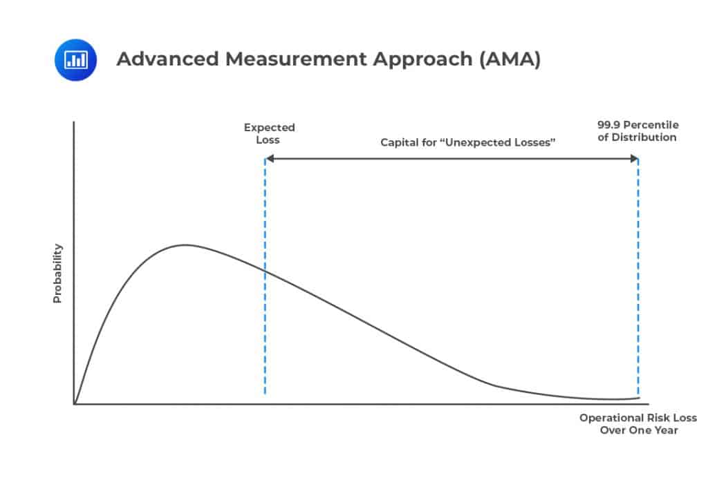
The AMA approach is much more complicated compared to other approaches. Under this method, the banks are required to treat operational risk as credit risk and set the capital equal to the 99.9 percentile of the loss distribution less than the expected operational loss, as shown by the figure below.
 Moreover, under the AMA approach, banks are required to take into consideration every combination of the eight business lines mentioned in the standardized approach. Combining the seven categories of operational risk with the eight business lines gives a total of (7 × 8 =) 56 potential sources of operational risk. The bank must then estimate the 99.9 percentile of one-year loss for each combination and then aggregate each combination together to determine the total capital requirement.
To use the AMA method, a bank has to satisfy all the requirements under the standardized approach, but the bank must also:
Currently, the Basel Committee has replaced the three approaches with a new standardized measurement (SMA) approach. Despite being abandoned by the Basel Committee, some aspects of the AMA approach are still being used by some banks to determine economic capital.
The AMA approach opened the eyes of risk managers to operational risk. However, bank regulators found flaws in the AMA approach in that there is a considerable level of variation in the calculation done by different banks. In other words, if different banks are provided with the same data, there is a high chance that each will come up with different capital requirements under the AMA.
The Basel Committee announced in March 2016 to substitute all three approaches for determining operational risk capital with a new approach called the standardized measurement approach (SMA).
The SMA approach first defines a quantity termed as Business Indicator (BI). BI is similar to gross income, but it is structured to reflect the size of a bank. For instance, trading losses and operating expenses are treated separately so that they lead to an increase in BI.
The BI Component for a bank is computed from the BI employing a piecewise linear relationship. The loss component is calculated as:
$$ 7\text{X}+7\text{Y}+5\text{Z} $$
Where X, Y, and Z are the approximations of the average losses from the operational risk over the past ten years defined as:
The computations are structured so that the losses component and the BI component are equal for a given bank. The Basel provides the formula used to calculate the required capital for the loss and BI components.
Computations of the economic capital require the distributions for various categories of operational risk losses and the aggregated results. The operational risk distribution is determined by the average loss frequency and loss severity.
The term “average loss frequency” is defined as the average number of times that large losses occur in a given year. The loss frequency distribution shows just how the losses are distributed over one year, specifying the mean and variance.
If the average losses in a given year are \(\lambda\), then the probability of \(n\) losses in a given year is given by Poisson distribution defined as
$$ \text{Pr}\left( \text{n} \right) =\cfrac { { \text{e} }^{ -\lambda }{ \lambda }^{ \text{n} } }{ \text{n}! } $$
The average number of losses of a given bank is 6. What is the probability that there are precisely 15 losses in a year?
From the question, \(\lambda=6\) . Therefore,
$$ \text{Pr}\left( 15 \right) =\cfrac { { \text{e} }^{ -6 }{ 6 }^{ 15 } }{ 15! } \approx 0.001 $$
Loss severity is defined as a probability distribution of the size of each loss. The mean and variance of the loss severity are modeled using the lognormal distribution. That is, suppose the standard deviation of the loss size is σ, and the mean is μ, then the mean of the logarithm of the loss size is given by:
$$ \text{ln}\left( \cfrac {\mu}{ \sqrt { 1+\text{w} } } \right) $$
The variance is given by:
$$ ln\left(1+ \text w\right) $$
Where:
$$\text{w}={ \left( \cfrac { \sigma }{ \mu } \right) }^{ 2 }$$
The estimated mean and standard deviation of the loss size is 50 and 20, respectively. What is the mean and standard deviation of the logarithm of the loss size?
We start by calculating w,
$$\text{w}={ \left( \cfrac { 20 }{ 50 } \right) }^{ 2 }=0.16$$
So the mean of the logarithm of the loss size is given by:
$$ \text{ln}\left( \cfrac { \mu}{ \sqrt { 1+\text{w} } } \right) =\text{ln}\left( \cfrac { 50 }{ \sqrt { 1.16 } } \right) =3.8378$$
The variance of the logarithm of the log size is given by:
$$\text{ln}\left(1+\text{w}\right)=\text{ln} \left(1.16\right)=0.1484$$
After estimating \(\lambda\), \(\mu\), and \(\sigma\), Monte Carlo simulation can be utilized to determine the probability distribution of the loss as illustrated below:
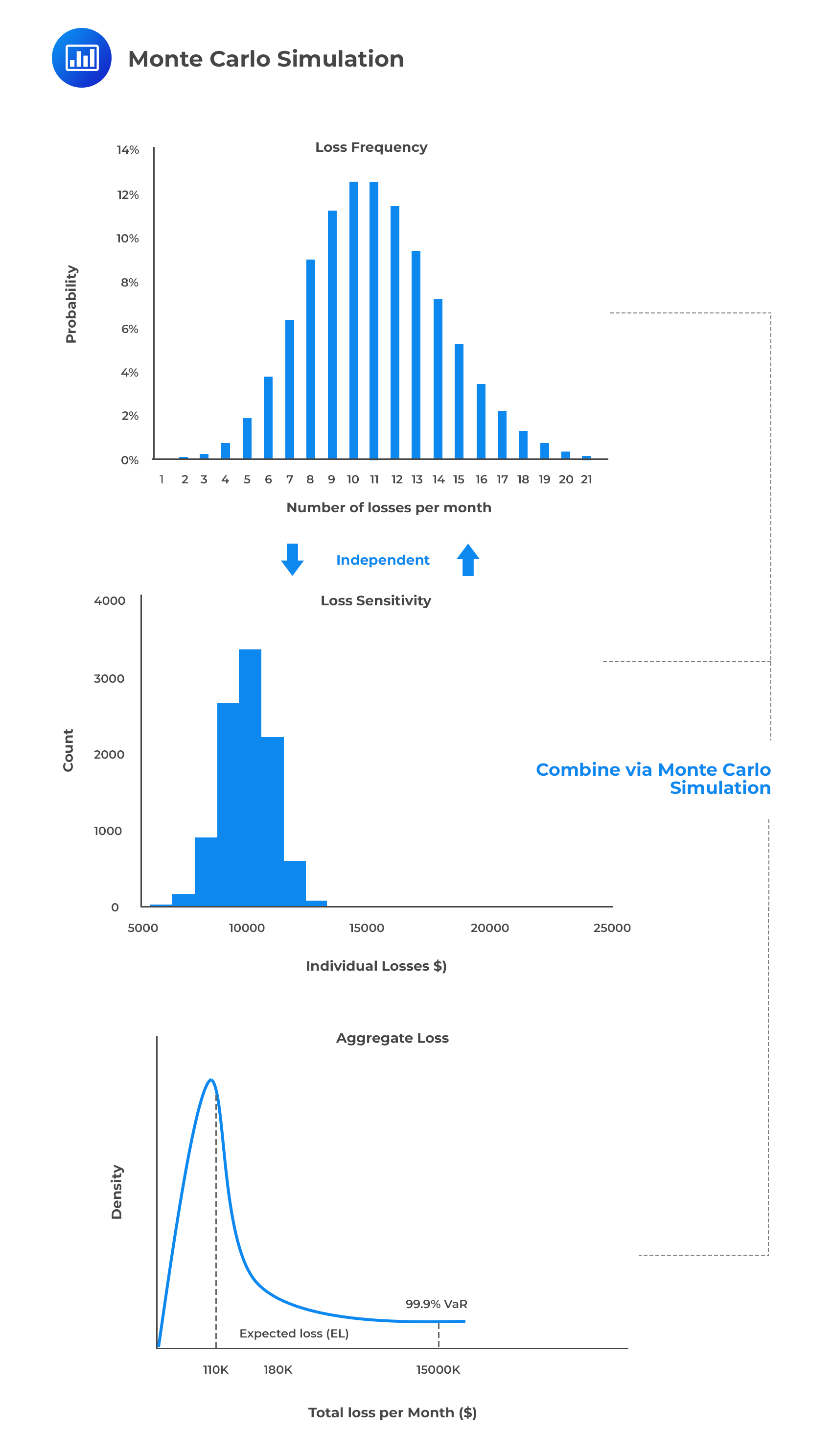 The necessary steps of the Monte Carlo Simulations are as follows:
Assume the average loss frequency is six, and a number sampled in step I is 0.29. Therefore, 0.29 corresponds to three loss events in a year because using the formula.
$$ \text{Pr}\left( \text{n} \right) =\cfrac { { \text{e} }^{ -\lambda }{ \lambda }^{ \text{n} } }{ \text{n}! } \\ \text{Pr}\left( 0 \right) +\text{Pr}\left( 1 \right) +\text{Pr}\left( 2 \right) =0.284\text{ and }\text{Pr}\left( 0 \right) +\text{Pr}\left( 1 \right) +\text{Pr}\left( 2 \right) +\text{Pr}\left( 3 \right) =0.4660 $$
Therefore 0.29 lies in between two cumulative probabilities.
Also, assume that the loss size has a mean of 60 and a standard deviation of 5 using the formulas \(\text{ln}\left( \cfrac {\mu}{ \sqrt { 1+\text{w} } } \right) \) and \( \text{ln} \left({ 1+\text{w} }\right) \).
In step II we will sample three times from the lognormal distribution using the mean
$$ \text{ln}\left( \cfrac { 60}{ \sqrt { 1+{ \left( \cfrac { 5 }{ 60 } \right) }^{ 2 } } } \right) =4.0909 \text{ and standard deviation} \text{ ln} \left( 1+{ \left( \cfrac { 5 }{ 60 } \right) }^{ 2 } \right) =0.0069$$
Now, assume the sampled numbers are 4.12, 4.70, and 5.5. Note that the lognormal distribution gives the logarithm of the loss size. Therefore we need to exponentiate the sampled numbers to get the actual losses. As such, the three losses are \({\text{e}}^{4.12}\)=61.56, \({\text{e}}^{4.70}\)=109.95 and \({\text{e}}^{5.5}\)=244.69.
This gives the total loss of 416.20 (61.56+109.95+244.69) in the trial herein.
Step 4 requires that the same process be repeated many times to generate the probability distribution for the total loss, from which the desired percentile can be computed.
The estimation of the loss frequency and loss severity involves the use of data and subjective judgment. Loss frequency is estimated from the banks’ data or subjectively estimated by operational risk professionals after considering the controls in place.
In the case that the loss severity cannot be approximated from the bank’s data, the loss incurred by other financial institutions may be used as a guide. The methods by which banks share information have been laid out. Moreover, there exist data vendor services (such as Factiva), which are useful at supplying data on publicly reported losses incurred by other banks.
The generally accepted scale adjustment for firm size is as follows:
$$ \text{Estimated Loss for Bank A} \\ = \text{Observed Loss for Bank B} \times \left( \cfrac {\text{Bank A Revenue}}{\text{Bank B Revenue}} \right)^{0.23} $$
Suppose that Bank A has revenues of USD 20 billion and incurs a loss of USD 500 million. Another bank B has revenues of USD 30 billion and experiences a loss of USD 300 million. What is the estimated loss for Bank A?
$$ \begin{align*} \text{Estimated Losss for Bank A} & = \text{Observed Loss for Bank B} \times \left( \cfrac {\text{Bank A Revenue}}{\text{Bank B Revenue}}\right)^{0.23} \\ &=300 \times \left( \cfrac {20}{30} \right)^{0.23} = \text{USD } 273.29 \text{ million}. \end{align*} $$
Scenario analysis aims at estimating how a firm would get along in a range of scenarios, some of which have not occurred in the past. It’s particularly essential when modeling low-frequency high-severity losses, which are essential to determine the extreme tails of the loss distribution.
The objective of the scenario analysis is to list events and create a scenario for each one. Scenarios considered come from:
For each scenario, loss frequency and loss severity are approximated. Monte Carlo simulations are used to determine a probability distribution for total loss across diverse types of losses. The loss frequency estimates should capture the existing controls at the financial institution and the type of business.
Estimation of the probability of rare events is challenging. One method is to state several categories and ask operational risk experts to put each loss into a category. For instance, some of the categories might be a scenario that happens once every 1,000 years on average, which is equivalent to \(\lambda=0.001\). The bank could also use a scenario happening once every 100 years on average, which is equivalent to \(\lambda=0.01\), and so on.
Operational risk experts estimate the loss severity, but rather than in the form of the mean and standard deviation, it is more suitable to estimate the 1 percentile to 99 percentile range of the loss distribution. These estimated percentiles can be fitted with the lognormal distribution. That is, if 1 percentile and 99 percentiles of the loss are 50 and 100 respectively, then 3.91 (ln(50)) and 4.61 (ln(100)) are 1 and 99 percentiles for the logarithm of the loss distribution, respectively.
The concluding point in scenario analysis is that it takes into consideration the losses that have never been incurred by a financial institution but can occur in the future. Managerial judgment is used to analyze the loss frequency and loss severity which can give hints on how such loss events may appear, which in turn assist the firms in setting up plans to respond to loss events or reduce the likelihood of it happening.
Typically, economic capital is allocated to business units, after which the return on capital is computed. Similar to credit risk, the same principles are used in the allocation of operational risk capital. The provision of operational risk capital to business units acts as an incentive to the business unit manager to reduce the operational risk because if the manager reduces the loss frequency and severity, less operational capital will be allocated. Consequently, the profit from the business unit will improve.
In a nutshell, the allocation of operational risk capital should sensitize the manager on the benefits of operational risk. Operational risk reduction does not necessarily reach an optimal point because there exists operational risk in a firm that cannot be avoided. Therefore, cost-benefit analysis is carried out when operational risk is reduced by increasing the operational cost.
The power-law states that, if v is the value of a random variable and that x is the highest value of v, then it is true that:
$$ \text{Pr}(\text{v}>\text{x})={ \text{Kx} }^{ {-}{\alpha} } $$
Where K and α are the parameters.
The power law holds for some probability distributions, and it describes the fatness of the right tail of the probability distribution of v. K is a scale factor, and α depends on the fatness of the right tail of the distribution. That is, the fatness of the right tail increases with a decrease in α.
According to the mathematician G.V Gnedenko, the power for many distributions increases as x tends to infinity. Practically, the power law is usually taken to be true for the values of x at the top 5% of the distribution. Some of the distributions in which the power-law holds to be true are the magnitude of earthquakes, trading volume of the stocks, income of individuals, and the sizes of the corporations.
Generally, the power-law holds for the probability distributions of random variables resulting from aggregating numerous independent random variables. Adding up the independent variables, we usually get a normal distribution, and fat tails arise when the distribution is a result of many multiplicative effects.
According to Fontnouvelle (2003), the power-law holds for the operational risk losses, which turns to be crucial.
A risk manager has established that there is a 95% probability that losses over the next year will not exceed $50 million. Given that the power law parameter is 0.7, calculate the probability of the loss exceeding (a) 20 million, (b) 70 million, and (c) 100 million.
According to the power law
$$\text{Pr}(\text{v}>\text{x})={ \text{Kx} }^{ {-} \alpha }$$
This implies from the question that,
$$ 0.05=\text{K}{ 50 }^{ -0.7 }\Rightarrow \text{K}=0.7731 $$
Thus,
$$ \text{P}(\text{v}>\text{x})={ 0.7731V }^{ -0.7 } $$
Now,
when x=20
$$ \text{p}(\text{v}>20)={ 0.7731\left( 20 \right) }^{ -0.7 }=0.09495 $$
when x=70
$$ \text{p}(\text{v}>20)={ 0.7731\left( 70 \right) }^{ -0.7 }=0.03951 $$
when x=100
$$\text{p}(\text{v}>100)={ 0.7731\left( 100 \right) }^{ -0.7 }=0.03071$$
It is crucial to measure operational risk and to compute the required amount of operational risk capital. However, it is also imperative to reduce the likelihood of significant losses and severity in case an event occurs. More often, financial institutions learn from each other. That is, if significant losses are incurred in one of the financial institutions, risk managers of other financial institutions will try and study what happened so that they can make necessary plans to avoid a similar event.
Some of the methods of reducing operational risk include: reducing the cause of losses, risk control, and self-assessment, identifying key risk indicators (KRI’s), and employee education.
Causal relationships describe the search for a correlation between firm actions and operational risk losses. It is an attempt to identify firm-specific practices that can be linked to both past and future operational risk losses. For example, if the use of new computer software coincides with losses, it is only wise to investigate the matter in a bid to establish whether the two events are linked in any way.
Once a causal relationship has been identified, the firm should then decide whether or not to act on it. This should be done by conducting a cost-benefit analysis of such a move.
Risk and control self-assessment (RCSA) involves asking departmental heads and managers to single out the operational risks in their jurisdiction. The underlying argument is that unit managers are the focal point of the flow of information and correspondence within a unit. As such, they are the persons best placed to understand the risks pertinent to their operations.
Some of the approaches RCSA methods include:
RCSA should be done periodically, such as yearly. The problem with this approach is that managers may not divulge information freely if they feel they are culpable or the risk is out of control. Also, a manager’s perception of risk and its potential rewards may not conform to the firm-wide assessment. For these reasons, there is a need for independent review.
Key risk indicators seek to identify firm-specific conditions that could expose the firm to operational risk. KRIs are meant to provide firms with a system capable of predicting losses, giving the firm ample time to make the necessary adjustments. Examples of KRIs include:
The hope is that key risk indicators can identify potential problems and allow remedial action to be taken before losses are incurred.
It is essential to educate the employees on the prohibited business practices and breeding risk culture where such unacceptable practices might be executed. Moreover, the legal branch of a financial institution educates the employees to be cautious when writing emails and answering phone calls. Essentially, employees should be mindful that their emails and recorded calls could become public knowledge.
Earlier in the reading, we saw that a bank using the AMA approach could reduce its capital charge, subject to extensive investment in operational risk management. One of the ways through which a bank can achieve this is by taking an insurance cover. That way, the firm is eligible for compensation if it suffers a loss emanating from a covered risk.
For all its advantages, taking an insurance policy comes with two problems:
In a bid to tame the moral hazard problem, insurers use a range of tactics. These may include deductibles, coinsurance, and policy limits. Stiff penalties may also be imposed in case there is indisputable evidence of reckless, unrestricted behavior.
A firm can intentionally keep insurance cover private. This ensures that its traders do not take unduly high-risk positions.
On matters trading, firms with poor internal controls are more likely to take up insurance policies compared to firms with robust risk management frameworks. To combat adverse selection, an insurer has to go to great lengths toward understanding a firm’s internal risk controls. The premium payable can then be adjusted to reflect the risk of the policy.
Question
Question 1
Melissa Roberts, FRM, has observed 12 losses in her portfolio over the last four years. She believes the frequency of losses follows a Poisson distribution with a parameter λ. The probability that she will observe a total of 4 losses over the next year is closest to:
A. 17%
B. 16%
C. 20%
D. 0.53%
The correct answer is A.
We need to find the parameter \(\lambda\), which from the questions we have,
$$ \lambda =\cfrac { 12 \text{ losses} }{ 4 \text{ years} } =3\text{ losses per year} $$
The probability of n losses in a given year is given by Poisson distribution, defined as
$$ \begin{align*} \text{Pr}\left( \text{n} \right) & =\cfrac { { \text{e} }^{ -\lambda }{ \lambda }^{ \text{n} } }{ \text{n}! } \\ \text{Pr}\left( \text{n} =4 \right) & =\cfrac { { \text{e} }^{ -3 }{ 3 }^{ 4 } }{ 4! } =0.168 \\ \end{align*} $$
Question 2
According to the Basel Committee, a bank has to satisfy certain qualitative standards to be allowed to use the advanced measurement approach when computing the economic capital required. Which of the following options is NOT one of the standards?
A. The bank must have a system capable of allocating economic capital for operational risk across all business lines in a way that creates incentives for these business lines to manage operational risk better.
B. Internal and external auditors must regularly and independently review all operational risk management processes. The review must include the policy development process and independent scrutiny of the risk management function.
C. The bank’s operational risk measurement system should only make use of internally generated data to avoid the bias associated with external data.
D. The bank must have an operational risk management function tasked with identification, assessment, monitoring, and control of operational risk.
The correct answer is C.
The Basel committee does not rule out the use of external data by banks. In fact, the committee recommends the use of a combination of both external and internal data to estimate the unexpected loss. External data may not conform to a particular firm, but firms are allowed to scale the data to fit their profiles. In some cases, internal data may be either insufficient or entirely unavailable, forcing the firm to look elsewhere.
Offered by AnalystPrep


