Properties of Interest Rates

After completing this reading, you should be able to:

• Describe the various categories of interest rates (Treasury rates, LIBOR, Secured Overnight Financing Rate (SOFR) and repo rates, Swaps, and explain what is meant by the “risk-free” rate).
• Calculate the value of an investment using different compounding frequencies.
• Convert interest rates based on different compounding frequencies.
• Calculate the theoretical price of a bond using spot rates.
• Calculate the Macaulay duration, modified duration, and dollar duration of a bond.
• Evaluate the limitations of duration and explain how convexity addresses some of them.
• Calculate the change in a bond’s price given its duration, its convexity, and a change in interest rates.
• Derive forward interest rates from a set of spot rates.
• Derive the value of the cash flows from a forward rate agreement (FRA).
• Calculate zero-coupon rates using the bootstrap method.
• Compare and contrast the major theories of the term structure of interest rates.

What is an Interest Rate?

An interest rate is a return earned by a lender on funds given out to a borrower.

Interest rates are expressed in basis points (1 basis point = 0.01%); which also implies that an interest rate of 2% is equal to 200 basis points.

Categories of Interest Rates

Treasury Rates

Treasury rates are the rates earned by investors in instruments used by a government to borrow in its own currency. These include Treasury bonds and Treasury bills. Treasury rates are considered “risk-free” because they have zero risk exposure. That has much to do with the ability of the government to use a range of tools at its disposal to avoid default, including printing of cash and increased taxes. T-bill and T-bond rates are used as the benchmark for nominal risk-free rates.

LIBOR

LIBOR, the London Interbank Offered Rate, is the rate at which the world’s leading banks lend to each other for the short term. It’s the most widely used benchmark for short-term lending.

Libor rates are compiled from the estimates of unsecured borrowing rates of 16 highly rated global banks. The rates are estimated daily for five different currencies. Libor has seven borrowing periods ranging from one day to one year.

Repo Rates

Repo rates are the implied rates on repurchase (repo) agreements. A repo agreement is an agreement between two parties – the seller and the buyer – where the seller agrees to sell a security to the buyer with the understanding that they (seller) will buy it back later at a higher price. The most common repo transactions are carried out overnight. The credit risk in a repo agreement depends on the term of the agreement as well as the creditworthiness of the seller.

Overnight Interbank Borrowing

The overnight interbank borrowing rate is the rate at which banks borrow from each other. Banks with excess reserves will lend to banks that have shortages. Cash reserves are kept at the central bank and are dependent on the liabilities of a bank. This type of borrowing occurs overnight. The overnight interbank rate, known as the fed funds rate in the US, is the main mechanism through which US monetary policy is channeled.

Swaps

Swaps are used to create long-term interest rates from short-term interest rates.

Assume two traders X and Y. A swap occurs when trader X agrees to pay trader Y a pre-determined fixed interest rate of 5% per year compounded quarterly, on a principal of say, $10,000, for five years. In return, trader Y agrees to pay trader X interest at the three-month Libor rate on the $10,000 principal for five years. Except for the first Libor rate, the Libor rates are unknown when the swap is agreed upon. In this example, interests will be exchanged every three months.

Risk-Free Rates

Risk-free rates are used in valuing derivatives. Overnight interbank rates determine the risk-free rates using overnight indexed swaps. Even though treasury rates are risk-free rates, they are not preferred since they are artificially low.

Compounding Frequencies

Given an initial investment of \(A\) that earns an annual rate \(R\), compounded \(m\) times a year for a total of \(n\) years, then we can compute the future value, \(FV\), as follows:

$$ FV=A{ \left( 1+\frac { R }{ m } \right) }^{ m\times n } $$

In the presence of continuous compounding, then:

$$ FV=A{ e }^{ R\times n } $$

Example: Future Value

Suppose USD 1,000 is invested for five years at an interest rate of 4% compounded quarterly per annum.

The future value of the fund after 5 years is given by

$$ \begin{align*}\text{FV}&=A{ \left( 1+\frac { R }{ m } \right) }^{ m\times n }\\ &  =1,000{ \left( 1+\frac { 0.04}{ 4 } \right) }^{ 20}=\text{USD 1,220.19}\end{align*}$$

Exam tip: For any rate \(R\), the future value with continuous compounding will always be greater than the future value with discrete compounding.

Let \({ R }_{ c }\) be the continuously compounded rate that equates the future value under discrete compounding to the future value under continuous compounding:

$$\begin{align*} A{ \left( 1+\frac { R }{ m } \right) }^{ m\times n }&=A{ e }^{ { R }_{ c }\times n }\\ { R }_{ c }&=m\times ln\left( 1+\frac { R }{ m } \right) \\ \end{align*}$$

Alternatively, given \({ R }_{ c }\),

$$ \begin{align*}R=m\left( { e }^{ \cfrac { { R }_{ c } }{ m } }-1 \right) \\ \end{align*}$$

Illustration: Different Compounding Frequencies

The table below shows the different future values when $50,000 is compounded at different compounding frequencies at the rate of 5% for three years.

$$\begin{array}{l|c|c}{\textbf{Compounding}\\ \textbf{Frequency}} & \textbf{Formula} & \textbf{Future Value} \\ \hline\text{Annual} & 50,000(1+0.05)^{1×3} & 57881.25 \\ \text{Semi-Annual} & 50,000(1+0.05/2)^{2× 3} & 57984.67 \\ \text{Quarterly} & 50,000(1+0.05/4)^{4× 3} & 58037.73 \\ \text{Monthly} & 50,000(1+0.05/12)^{12× 3} & 58073.61 \\ \text{Daily} & 50,000(1+0.05/365)^{365× 3} & 58091.12 \\ \text{Continuous} & 50,000×e^{0.05×3} & 58091.71\\ \end{array}$$

From the table above, we can see that continuous compounding gives a higher value than discrete compounding. We can also see that the higher the number of compounding frequencies for discrete compounding, the higher the amount

The Usual Conventions

Sometimes, compounding frequencies are determined based on the frequency of payments. Interests of money market instruments – instruments with maturities of less than one year – are expressed as quarterly if payment occurs after three months. If payments occur after six months, they are expressed as semiannual, and as annual if they occur yearly.

Discounting

Discounting is the process of determining the present value of a known future amount.

The general discounting formula is:

$$ PV=A(1+\frac{R}{m})^{-mn} $$

Where:

• PV is the present value of an amount A,
• R is the interest rate compounded with a frequency of m times a year,
• m is the frequency by which R is compounded, and
• n is the number of years.

Also note that \((1+\frac{R}{m})^{-mn}\) is known as the discount factor.

Example: Present Value

Suppose an amount X is invested for five years at an interest rate of 4% compounded quarterly per annum. If the fund grows to USD 1,500 after 5 years, what is the value of X?

Solution

$$ PV=A(1+\frac{R}{m})^{-mn}=1,500(1+\frac{0.04}{4})^{-20}=\$1,229.32$$

The Theoretical Price of a Bond Using Spot Rates

The theoretical price of a bond is given by the present value of all of the bond’s cash flows. Assuming each cash flow is associated with a spot discount factor \({ z }_{ j }\), then:

$$ P = \sum_{j=1}^{n} \frac{C}{(1 + z_j)^T} + \frac{FV}{(1 + z_j)^n}$$

Where:

\(P\) = Sum of discounted cash flows.

\(C\) = Cash flow in each period.

\(z_j\) = discount rate for the \(j^{th}\) period.

\(T\) = time or period.

\(FV\) = future value.

The yield of a bond is the single discount rate that equates the bond’s present value to its market price. A bond’s par yield is the discount rate that equates the bond’s price to its par value.

Example

Consider a $1,000 face value, two-year bond that pays a coupon rate of 10% semi-annually, and that a spot rate of 11% compounded semi-annually, applies to each cash flow.

The price of the bond, in this case, is given by,

$$P = \frac{50}{1.055^1} + \frac{50}{1.055^2} + \frac{50}{1.055^3} + \frac{50}{1.055^4} + \frac{1000}{1.055^4} = \text{USD 982.47}$$

Duration Measures

Duration

Duration, sometimes referred to as Macaulay duration, is an approximate measure of a bond’s price sensitivity to changes in interest rates. 

Duration is expressed in years. For a zero-coupon bond, its duration is simply its time to maturity. For a coupon bond, its duration is shorter than maturity because the cash flows have different weights. $$\text{Macaulay Duration}=\frac{\sum_{t=1}^{n}\text{PV}(C_{t})T} {\text{Market Price of Bond}}$$ Where \(\text{PV}(C_{t})\) is the present value of coupon payments at time t, and T is the time to maturity

The formula for Macaulay duration, given continuous compounding, is:

$$ \text{ Macaulay Duration }={ \Sigma }_{ i=1 }^{ n }{ t }_{ i }\left[ \frac { { c }_{ i }{ e }^{ -y{ t }_{ i } } }{ P } \right] $$

Where:

\({ t }_{ i }\)=time in years until cash flow \({ c }_{ i }\) is received

\(y\)=the continuously compounded yield (discount rate) based on a bond price \(P\)

Example: Macaulay Duration

Consider a bond  whose current price is USD 120 with a cash flow in one year providing a present value of USD 20 and a cash flow in two years providing a present value of USD 100, the Macaulay duration, in this case, is given by:

$$\frac { 20 }{ 120 }\times 1+\frac { 100 }{ 120 }\times 2=1.8333$$

Modified Duration

Modified duration is used in the absence of continuous compounding of the yield. If the yield, \(y\), is expressed as a rate compounded \(n\) times a year, then:

$$ \text{Modified duration}=\left[ \frac { \text{Macaulay duration} }{ \left( 1+\frac { y }{ n } \right) } \right] $$

Note: By yield, we imply the yield to maturity.

Modified duration is based on the concept that bond prices have an inverse relationship with interest rates. When interest rates rise, bond prices fall; when interest rates fall, bond prices rise. Modified duration tells how much a bond’s price will rise or fall for a 1% shift in yield to maturity. 

Let’s say a bond has a modified duration of 5%. What does that imply? Its price will rise by about 5% if its yield drops by 1% (100 basis points), and its price will fall by about 5% if its yield rises by 1%.

Example: Modified Duration

Consider the bond in the previous example, and suppose that the yield with semi-annual compounding is 5 %.

The modified duration is thus given by:

$$\frac { 1.8333 }{ 1+\frac { 0.05}{2}}=1.7886$$

Exam tip: Unless given, you must calculate the Macaulay duration to determine the modified duration.

Dollar Duration

The dollar duration, DD, of a bond is a product of its modified duration and its market price. If we use \({ D }^{ \ast }\) to denote the modified duration, and \({ P }_{ 0 }\) to denote the bond’s market price, then:

$$ DD={ D }^{ \ast }\times { P }_{ 0 } $$

For illustration, consider the bond in the example above, the dollar duration is given by,

$$120 \times1.7886=214.63 $$

Limitation of Duration

Note that the approximate duration relationship is given by:

$$\Delta P=-DP\Delta y ………………….1$$

Which is equivalent to,

$$\frac{\Delta P}{P}=-D\Delta y $$

Where,

\(P=\) price of the bond

\(D=\) bond’s duration

\(\Delta P=\) change in bond’s price

\(\Delta y=\) change in bond’s yield

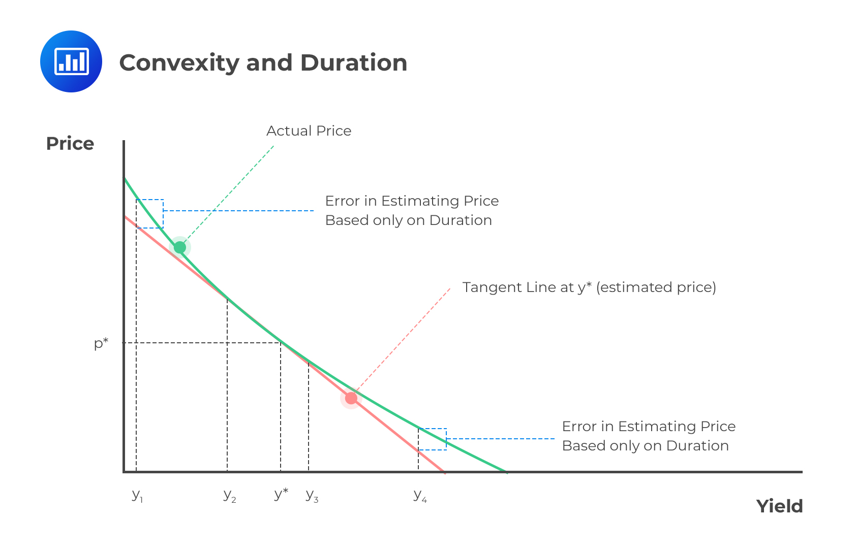
Duration provides a good approximation of the effect of a small parallel shift in the interest rate term structure. However, the above duration relationship cannot provide a good approximation in case the change in the bond yield arises from a non-parallel shift in the interest rate term structure or if the change being considered is large.

This problem is addressed by convexity.

Convexity

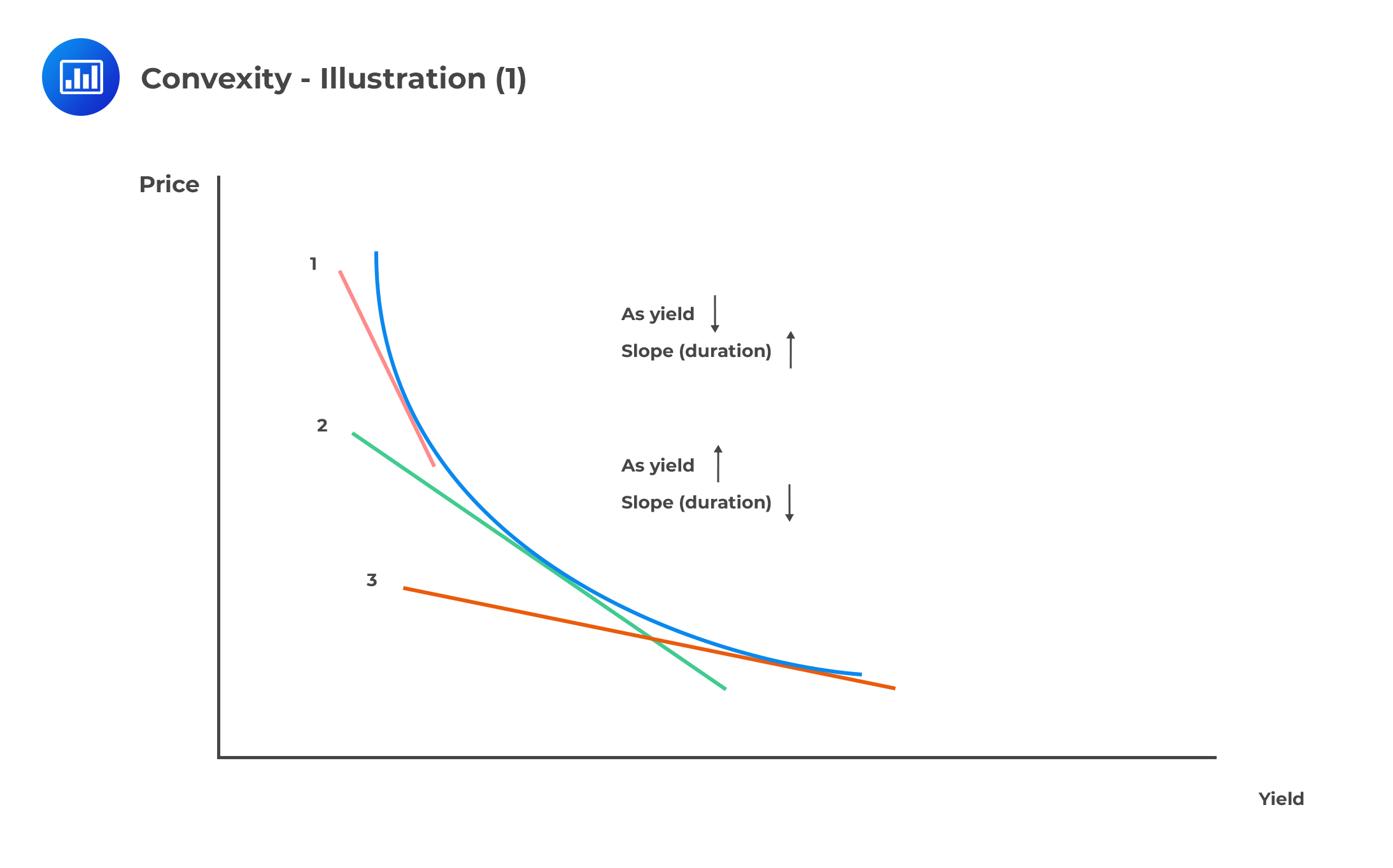
Convexity is a measure of the curvature in the relationship between bond prices and bond yields. It demonstrates how the duration of a bond changes as the interest rate changes. Convexity estimates the amount of market risk affecting a bond or portfolio.

If we let C be the convexity, then equation 1 above can be refined so that we have:

$$\Delta P=-DP\Delta y +\frac{1}{2}CP(\Delta y)^2$$

With this equation, relatively large parallel shifts can now be considered.

If bond \(X\) has a higher convexity than bond \(Y\), what does this imply? All else being equal, bond \(X\) will always have a higher market price than bond \(Y\) as interest rates rise and fall.

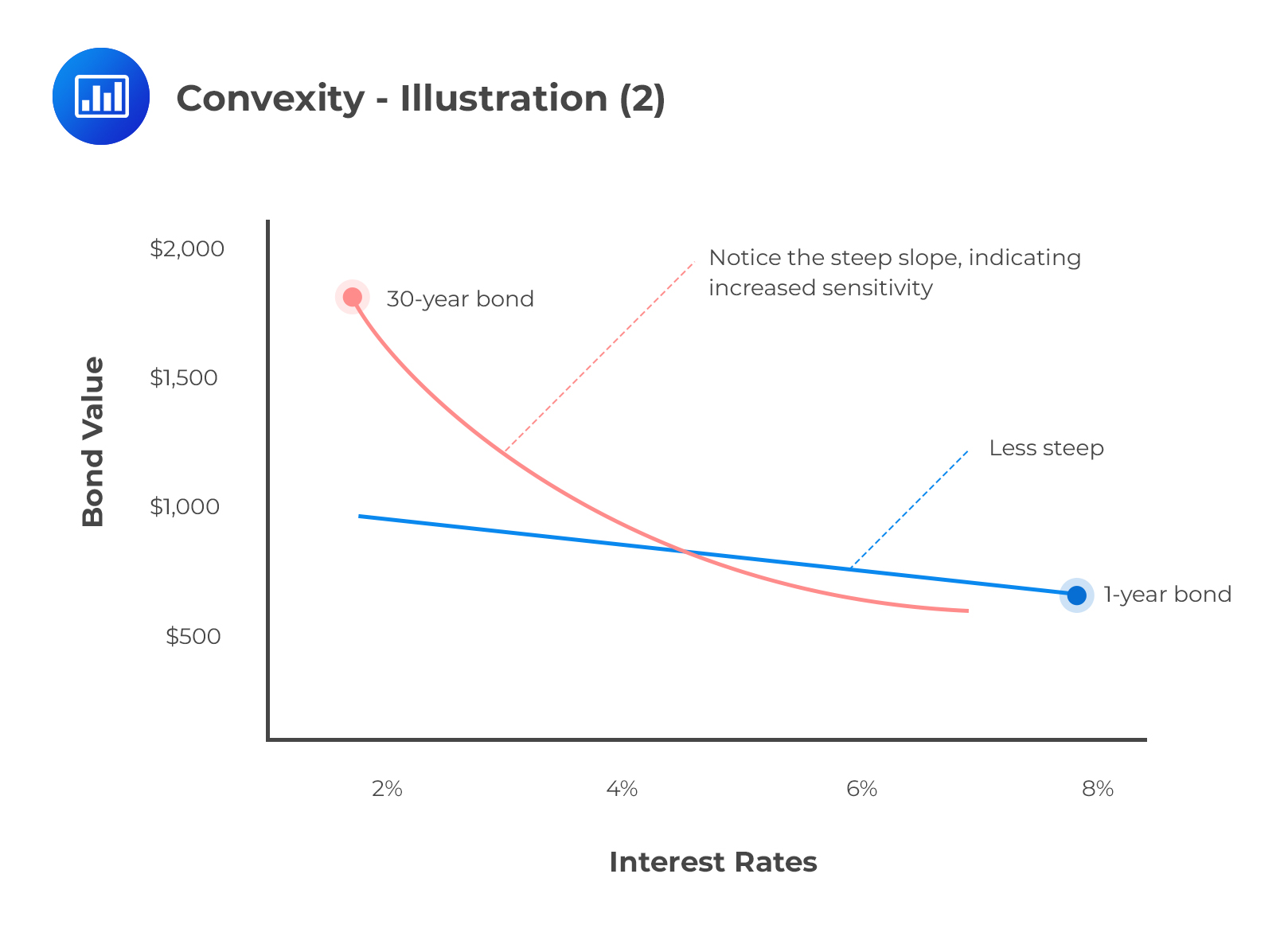Duration assumes that interest rates and bond prices have a linear relationship. It’s, therefore, a fairly good measure of exactly how bond prices are affected by small changes in interest rates. However, the relationship between bond prices and interest rates is actually non-linear, i.e., convex. This makes convexity a better measure of risk, especially in the presence of large and frequent fluctuations in interest rates.

For the purpose of the percentage change in price triggered by convexity, i.e., the price change not explained by duration, we must calculate the convexity effect.

$$ \text{Convexity effect}=\frac { 1 }{ 2 } \times \text{Convexity} \times \Delta { y }^{ 2 } $$

Exam tip: Convexity is always positive for regular coupon-paying bonds

Calculating the Change in a Bond’s Price Given Its Duration, Its Convexity, and a Change in Interest Rates

Combining duration and convexity results in a far more accurate estimate of the change in the price of a bond given a change in yield.

$$\begin{align*} \text{Change in bond’s price} &= \text{Duration effect} + \text{Convexity effect}\\  &=\left[ –\text{Duration} \times \text{Price} \times \text{Change in yield} \right] \\ & +\left[ \cfrac { 1 }{ 2 } \times \text{Convexity} \times \text{Price} \times \left( \text{Change in yield}  \right)^{ 2 } \right] \\ \end{align*}$$

Example: Change in a Bond’s Price

A portfolio manager has a bond position worth 100 million. The position has a modified duration of 3 years and a convexity of 60. Assuming that the term structure is flat, by how much does the value of the position change if interest rates increase by 25 basis points?

Solution

$$ \begin{align*}\text{Change in bond’s price}& = \text{Duration effect}  + \text{Convexity effect}\\ & =\left[ –\text{Duration} \times \text{Price} \times \text{Change in yield} \right] \\ & +\left[ \cfrac { 1 }{ 2 } \times \text{Convexity} \times \text{Price} \times { \left( \text{Change in yield}  \right) }^{ 2 } \right] \\ &=-3\times 100,000,000\times 0.0025 \\ &+\left[ 0.5\times 60\times 100,000,000\times { 0.0025 }^{ 2 } \right] \\ &=-731,250 \\ \end{align*}$$

With every increase in interest rates of 25 basis points, the bond’s price will decrease by $731,250

Deriving Forward Rates from a Set of Spot Rates

\({ y }_{ n }\), the \(n\)-year spot rate, is a measure of the average interest rate over the period from now until \(n\) years’ time.

The forward rate, \({ f }_{ t, t+r }\), is a measure of the average interest rate between times \(t\) and \(t + r\). It’s the interest rate agreed today \((t=0)\) on an investment made at time \(t>0\) for a period of \(r\) years.

The one-year forward rate, \({ f }_{ t, t+1 }\), is therefore the rate of interest from time \(t\) to time \(t +1\). It can be expressed in terms of spot rates as follows:

$$ 1+{ f }_{t, t+1} = \frac{{{(1+{y}_{t+1})}}^{t+1}}{{(1+{y}_{t})}^{t}} $$

If we want to find the forward rate for a period greater than 1-year, e.g., 2-year forward rate, then we will use the formula: $$\left(1+{ f }_{t, n}\right)^{n-t} = \frac{{{(1+{y}_{n})}}^{n}}{{(1+{y}_{t})}^{t}} $$ Where \({ y }_{ n }\), the \(n\)-year spot rate and \({ y }_{ t }\), the \(t\)-year spot rate. For example, consider a case where we want to calculate the forward rate between year 2 and year 4, that is, \(f_{2,4}\). In such a case, we will use the formula, $$f_{2,4}^{4-2}=\frac{(1+y_4)^4}{(1+y_2)^2}$$

The above results for 1-year forward rate can be generalised as follows,

Step 1: Use the formula:

$$ 1+F=\frac {V_2}{V_1} $$

Where \(V_1\) is the value to which a dollar grows by time \(T_1\) and \(V_2\) is the value to which a dollar grows by \(T_2\).

Step 2: Calculate the interest rate that equates the value of one dollar at time \(T_1\) to the value of one dollar at time \(T_2\).

Example: Semiannual Forward Rates

Assume that the six-month spot rate is 0.05, while the one-year spot rate is 0.058. Calculate the forward rate for the period between six months and one year.

To get the forward rate, we take \(\frac {V_2}{V_1}\):

$$ \begin{align*}V1&=(1+\frac {0.05}{2})=1.025 \\ V2&=\left(1+\frac{0.058}{2}\right)^2 =1.058841 \\ \end{align*}$$

\(\frac {V_2}{V_1}\) is therefore \(\frac {1.058841}{1.025} = 1.033\).

The interest rate at which one dollar has grown between the two periods is \(1.033-1=0.033\).

If the forward rate is expressed with semiannual compounding:

$$\begin{align*} F/2&=0.033\\ F&= 0.066\\ \end{align*}$$

Therefore the forward rate is 6.6% expressed with semiannual compounding

Annual Forward Rates

Let’s say you have the following spot rates table:

$$\begin{array}{l|cccc} \textbf{Year} & 1 & 2 & 3 & 4\\ \hline \textbf{Spot Rate} & 1.2\% & 1.5\% &1.9\% & 2.4\% \end{array}$$

The one-year forward rate between years 1 and 2 is:

$$\begin{align*}1+{ f }_{1, 2}&=\frac {V_2}{V_1} = \frac { { { \left( 1+{ 1.5\% } \right) } }^{2 } }{ { \left( 1+{ 1.2\% } \right) }^{ 1 } } = 1.018\\  { f }_{ 1, 2 } &= 1.8\% \\ \end{align*}$$

In the same vein, we can calculate the one-year forward rate between years 3 and 4:

$$ \begin{align*}1+{ f }_{ 3, 4 }&=\frac {V_4}{V_3} = \frac { { { \left( 1+{ 2.4\% } \right) } }^{4 } }{ { \left( 1+{ 1.9\% } \right) }^{ 3 } } = 1.039\\ { f }_{ 3, 4 } &= 3.9\% \\ \end{align*}$$

Continuous Compounding

Take the example shown above. If the interest rate is expressed with continuous compounding:

$$ \begin{align*} V_1&=e^{R_1 T_1}\\ V_2&=e^{R_2 T_2}\\ \end{align*}$$

The forward rate, F, with continuous compounding between time \(T_2\) and time \(T_1\)  is thus:

$$ F=e^{F(T_2- T_1)}=\frac {V_2}{V_1}=e^{R_2 T_2 – R_1 T_1}$$

Rearranging the above gives the forward rate F as:

$$ F=\frac {R_2T_2-R_1T_1}{T_2-T_1} $$

Example: Continuous Compounding

Assume the data in the following spot rates table is continuously compounded:

$$ \begin{array}{lcccc} \text{Year} & 1 & 2 & 3 & 4 \\ \text{Spot rate} & 1.4\% & 1.8\% &2.1\% & 2.6\%\\ \end{array} $$

Calculate the continuously compounded forward rate between years 1 and 2.

$$ \begin{align*} F& = \frac{R_2 T_2 – R_1 T_1}{T_2-T_1}\\ &= \frac{0.018(2)-0.014(1)}{2-1}\\ & = 2.2\%\\ \end{align*}$$

As you can see, when dealing with continuous compounding, the spot rate is simply multiplied by the time period instead of using \((1+y_t)^t\).

Forward Rate Agreements

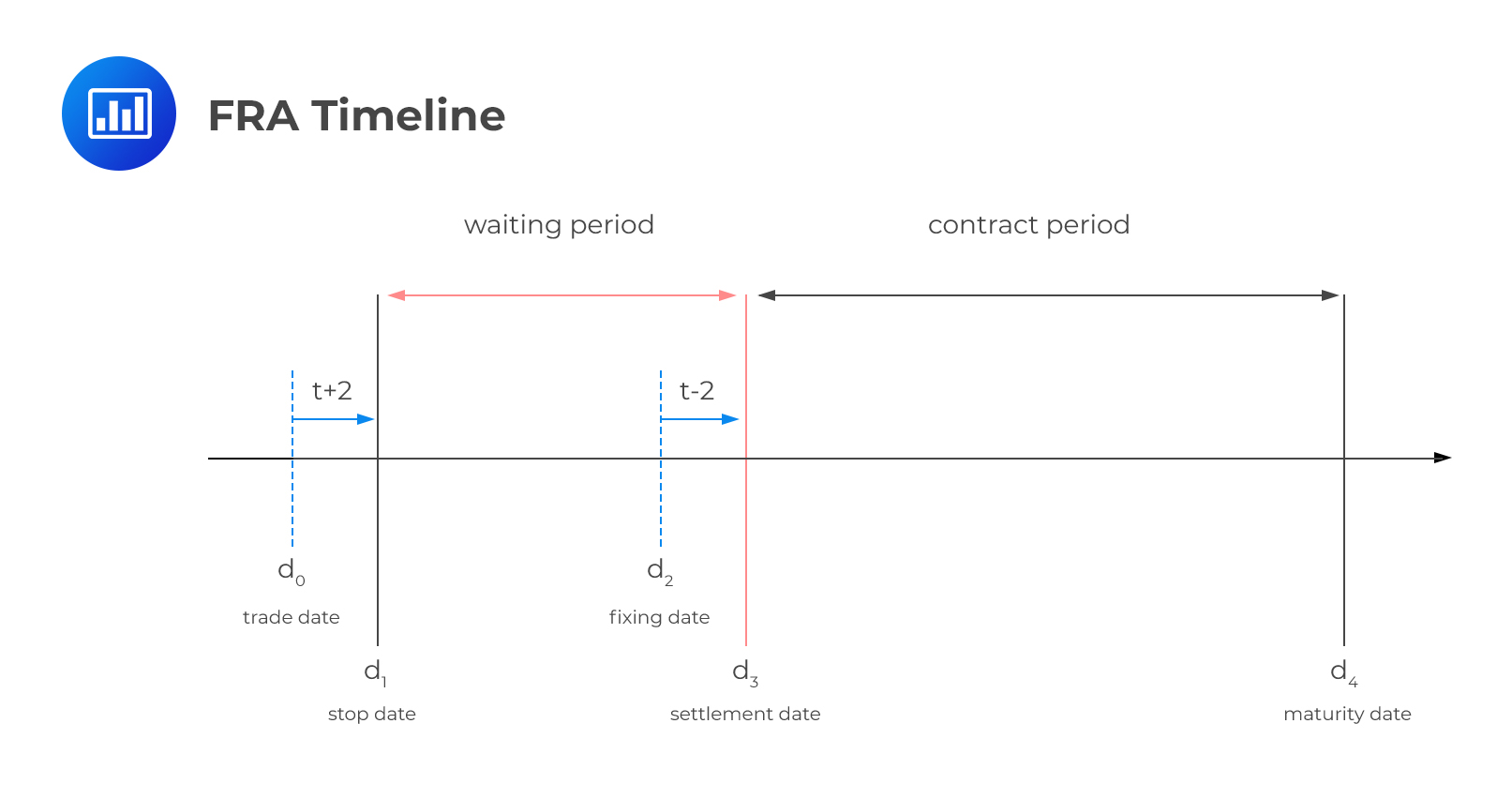
A forward rate agreement is an agreement between two parties to lock in an interest rate for a specified period of time starting on a future settlement date, based on a notional amount. The buyer of a forward rate agreement enters into the contract to protect himself from any future increase in interest rates. The seller, on the other hand, enters into the contract to protect himself from any future decline in interest rates. If Firm A and Firm B enter into a forward rate agreement by agreeing on an interest rate \(R_K\), the cash flows will be:

$$ \begin{align*} \text{Firm A: } &L(R_{K} – R_{M} )(T_{2} -T_{1}  ) \\ \text{Firm B: } &L(R_M-R_K )(T_2-T_1 )\\  \end{align*}$$

Where:

\(L\) = principal amount

\(R_K\) = interest rate agreed to in the FRA

\(R_M\) = actual interest rate observed between T1 and T2

FRAs are cash-settled on the settlement date – the start date of the notional loan or deposit. The interest rate differential between the market rate and the FRA contract rate determines the exposure to each party. It’s important to note that as the principal is a notional amount, there are no principal cash flows.

As time passed, the agreed fixed rate \(R_K\) remains the same but the forward LIBOR rate \(R_F\) is likely to move in either direction.

Therefore, the value of the forward contract to both parties will be:

$$ \begin{align*} \text{Firm A: } &V_{FRA} = L(R_{K} – R_{F} )(T_{2} -T_{1}  ) e^{- R_2 T_2}\\ \text{Firm B: } &= L(R_{F} – R_{K} )(T_{2} -T_{1}  ) e^{- R_2 T_2}\\ \end{align*} $$

Where:

\(V_{FRA}\) = value of the forward contract

\(R_2\) = the continuously compounded risk-free rate for a maturity \(T_2\)

Example: Forward-Rate Agreements

A German bank and a French bank entered into a semiannual forward rate agreement contract where the German bank will pay a fixed rate of 4.2% and receive the floating rate on the principal of €700 million. The forward rate between 0.5 years and 1 year is 5.1%. If the risk-free rate at the 1-year mark is 6%, then what is the value of the FRA contract between the two banks?

$$ \begin{align*} V_{FRA} &= L(R_{K} – R_{F} )(T_{2} -T_{1}  ) e^{- R_2 T_2}\\ &= €700 \text{million} (5.1\% – 4.2\%)(0.5 \text{years}) e^{-0.06 * 1 \text{year}}\\ &=3,056,903.43\end{align*} $$

Zero Rates

A zero-coupon interest rate is also known as zero-rate or spot rate. This is the interest rate that is applied when an investor receives the total return, i.e, interest, and principal at the maturity of the bond.

Bonds with maturities of less than one year provide zero rates directly since they provide total return, (interest and principal) at maturity. Bonds with maturities of more than one year, provide regular coupon payments prior to their maturity. Therefore, zero rates for such bonds have to be calculated.

Consider the following example for illustration,

Example: Zero Rates

Suppose the zero-coupon interest rates (semi-annually compounded) for maturities of 0.5, 1.0, and 1.5 years are 2.0%, 2.5% and 3.0%, respectively. Now consider a USD 1,000 face value, two-year bond that currently trades at 1020, and pays semi-annual coupons of 8%. If the two-year zero-coupon interest rate is R, then, R can be solved using the following equation:

$$\begin{align*}&\frac{40}{\left(1+\frac{0.02}{2}\right)^1}+\frac{40}{\left(1+\frac{0.025}{2}\right)^2}+\frac{40}{\left(1+\frac{0.03}{2}\right)^3}+\frac{1040}{\left(1+\frac{R}{2}\right)^4}=1,020 \\& \Rightarrow R=7.18\%\end{align*}$$

Theories of the Term Structure

Market Segmentation Theory

This theory argues that different maturity periods on interest-bearing instruments attract different traders. Traders interested in short-term maturity instruments will influence short-term maturity rates. The same is true for traders interested in medium- and in long-term maturity instruments.

Since traders do not focus on only one part of the interest rate term structure, this theory is considered to be unrealistic.

Expectations Theory

This theory argues that the interest rate term structure reflects the future market expectations of interest rates.

The interest rate term structure will have long-maturity rates being higher than short-maturity rates (upward sloping curve) if the market expects interest rates to rise. The opposite is true if the market expects interest rates to fall.

Liquidity Preference Theory

This theory argues that if the expectations theory holds, most investors will prefer short-term investments to long-term investments. This is because of liquidity considerations – the funds invested in short-term investments will be available earlier to meet any need.

Liquidity considerations create a mismatch between borrowers and lenders as it makes borrowers want to borrow for longer periods and lenders want to lend for shorter periods. Financial intermediaries attempt to fix this mismatch, and in so doing, supply and demand are matched at both maturities.

Question

A portfolio manager has a bond position worth CAD 200 million. The position has a modified duration of six years and a convexity of 120. Assuming that the term structure is flat, by how much does the value of the position change if interest rates increase by 50 basis points?

A. CAD -5,700,000

B. CAD -5,000,000

C. CAD -6,000,000

D. CAD -54,000,000

The correct answer is A.

$$ \begin{align*}\text{Change in bond’s price}& = \text{Duration effect}  + \text{Convexity effect}\\ & =\left[ –\text{Duration} \times \text{Price} \times \text{Change in yield} \right] \\ & +\left[ \cfrac { 1 }{ 2 } \times \text{Convexity} \times \text{Price} \times { \left( \text{Change in yield}  \right) }^{ 2 } \right] \\ &=-6\times 200,000,000\times 0.005 \\ &+\left[ 0.5\times 120\times 200,000,000\times { 0.005 }^{ 2 } \right] \\ &=-5,700,000 \\ \end{align*}$$

With every increase in interest rates of 50 basis point, the bond’s price will decrease by $5.7 million.