


Correlations and Copulas
After completing this reading you should be able to: Define correlation and covariance... Read More
After completing this reading you should be able to:
An external rating scale is a scale used as an ordinal measure of risk. The highest grade on the scale represents the least risky investments, but as we move down the scale, the amount of risk gradually increases (safety decreases).
An issue-specific credit rating conveys information about a specific instrument, such as a zero-coupon bond issued by a corporate entity. An issuer-specific credit rating, on the other hand, conveys information about the entity behind an issue. The latter usually incorporates a lot more information about the issuer.
Here are S&P’s and Moody’s credit rating scores for long-term obligations:
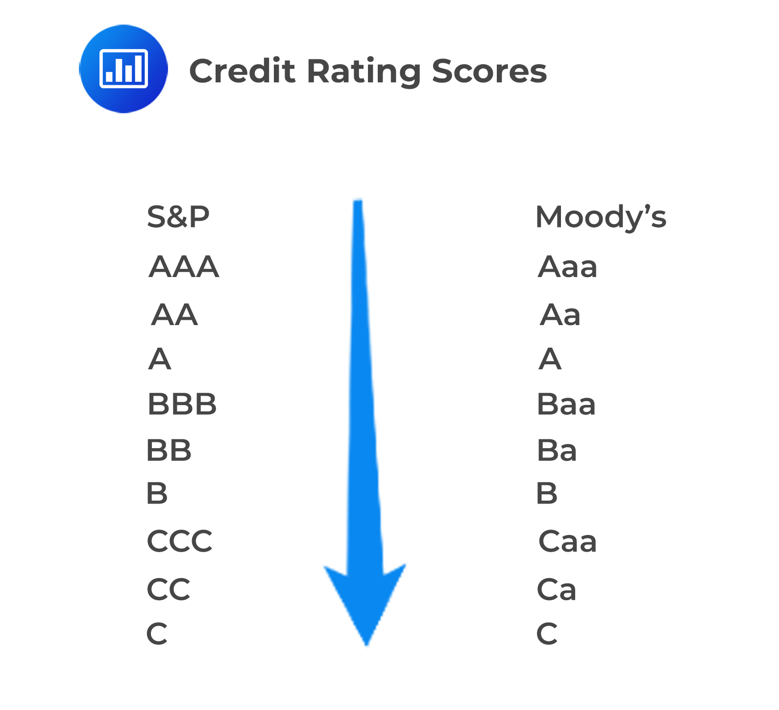 The successive move down the scale represents an increase in risk. In the case of Moody’s ratings, Baa and above are said to be investment-grade while those below this level are said to be non-investment-grade.
In the case of S&P’s, ratings BBB and above are investment-grade. All the others are non-investment-grade.
The process leading up to the issuance of a credit rating follows certain steps. These are:
Apart from the ratings themselves, the rating agencies also provide outlooks which shows the changes likely to be experienced over the medium term.
When a rating is placed on a watchlist, it shows that a very small short-term change is expected.
Rating stability is necessary since ratings are majorly used by bond traders. If the ratings were to change, then the bond traders are required to trade more frequently and, in this case, they are likely to incur a lot of transaction costs.
Rating stability is important because ratings are also used in financial contracts, and if the ratings vary for different bonds, it would be difficult to administer the underlying contracts.
The probability of default given any rating at the beginning of a cycle increases with the time horizon. Non-investment bonds are the worst hit. Their default probabilities can dramatically increase within a short time.
Since ratings are generally produced with an eye on a long-term period, they must take into account any economic/industrial cycle on the horizon. Rating agencies make efforts to incorporate the effects associated with an economic cycle in their ratings. Although this practice is generally valid, it can lead to underestimation or overestimation of default if the predicted economic cycle doesn’t play out exactly as expected. Put precisely, the probability of default can be underestimated if an economic recession occurs, or overestimated if an economic boom occurs. In addition, the default rate of lower-grade bonds is correlated with the economic cycle, while the default rate of high-grade bonds is fairly stable.
Two firms in different industries – say, banking and manufacturing – could have the same rating, but the probability of default may be higher for one of the firms than for the other. What does that mean? The implication here is that for a given rating category, default rates can vary from industry to industry. However, there’s little evidence to support the notion that geographic location has a similar effect.
Consider a firm defaulting in a very short time, that is, \({\delta }{\text t}\).
The task is to answer the question, “What is the conditional probability of a firm defaulting between time \(t\) and time \(t+{\delta}t\) given that there is no default before time \(t\)?”
We can denote this by \({h\delta}t\), where \(h\) is the rate at which defaults are happening at time \(t\) .
Unconditional default probabilities can be calculated using the hazard rates.
Suppose that \(\bar{h}\) is the average hazard rate between time \(0\) and time \(t\).
Then, the unconditional probability between time \(0\) and \(t\) is
$$ 1-\text{exp}\left(-{\bar{\text{h}}t}\right) $$
and the survival probability to time t is therefore given by
$$\text{exp}\left(-{\bar{\text{h}}t} \right)$$
and the unconditional probability between time \({\text{t}_1}\) and \({\text{t}_2}\) is given by the expression;
$$ \text{exp}\left(-\bar{\text{h}}_1\text{t}_1\right)-\text{exp}\left(-\bar{\text{h}}_2\text{t}_2\right) $$
Suppose you have been given a constant hazard of 0.05,
Calculate:
$$ \begin{align*} &1-\text{exp}\left( -\text{ht} \right) \\ =&1-\text{exp}\left(-0.05 \times 2\right) = 0.09516 \end{align*} $$
$$ \text{exp}\left(-0.05 \times 2 \right)-\text{exp}\left(-0.05 \times 3 \right)=0.04413 $$
$$\begin{align*}&\frac{\text{Unconditional probability of a default occurring during the third year}}{\text{Probability of surviving to the end of the second year}}\\&=\frac{0.04413}{1- 0.09516}=0.04877\end{align*}$$
In the event that a firm runs bankruptcy or defaults, it may pay part of the amount of the total loan to the lender. This amount that is repaid, expressed as a percentage, is known as the recovery rate.
Since the loan is not fully repaid, then we can calculate the expected loss from the loan over a given period of time as;
$$ \begin{align*} \text{Expected Loss}&= \text{Probability of Default} \times \text{Loss Given Default} \\ \text{EL} &= \text{PD} \times \text{LGD} \end{align*} $$
But since \(\text{LGD}=1-\text{Recovery Rate}\)
Then, the expected loss from a loan is also calculated as
$$ \text{EL}= \text{PD} \times \left(1-\text{Recovery Rate} \right) $$
For example, if the recovery rate is 70%, then
$$ \text{LGD}=100\%-70\%=30\%. $$
Suppose the debt instrument has a notional value of $100 million, and that there is a 1% probability of default, then the expected loss when the loan defaults is $0.3 million.
Point-in-time ratings, also called at-the-point internal ratings, evaluate the current situation of a customer by taking into account both cyclical and permanent effects. As such, they are known to react promptly to changes in the customer’s current financial situation.
Point-in-time ratings, try to assess the customer’s quantitative financial data (e.g. balance sheet information), qualitative factors (e.g. quality of management), and information about the state of the economic cycle. Using statistical procedures such as scoring models, all that information is transformed into rating categories.
Point-in-time ratings, are only valid for the short-term or medium term, and that’s largely because they take into account cyclic information. They are usually valid for a period not exceeding one year.
Through-the-cycle (ttc) internal ratings try to evaluate the permanent component of default risk. Unlike point-in-time ratings, they are said to be nearly independent of cyclical changes in the creditworthiness of the borrower. They are not affected by credit cycles, i.e. they are through-the-cycle. As a result, they are less volatile than at-the-point ratings and are valid for a much longer period (exceeding one year).
Advantages of ttc ratings include:
One of the disadvantages of ttc ratings over at-the-point ratings is that they can at times be too conservative if the stress scenarios used to develop the rating are frequently materially different from the firm’s current condition. If the firm’s current condition is worse than the stress scenarios simulated, then the ratings may be too optimistic. In fact, ttc ratings have very low default prediction in the short-term.
Apart from the commonly known rating agencies, that is, Moody’s, S&P, and Fitch, we have some organizations such as KMV and Kamakura which use some models to come up with default probabilities and hence can then use probabilities to provide important information to clients.
Factors considered include:
In the underlying model, a company defaults if the value of its debt exceeds the value of its assets.
Suppose \(v\) is the value of the asset and \(d\) is the value of the debt, the firm defaults when \( {\text{v}} < {\text{d}} \).
The value of the equity, at a future point in time, is:
$$ \text{Equity}= \text{max}\left( \text{v-d},0 \right) $$
This implies that equity in a company is a call option on the assets of the firm with a strike price equal to the face value of the debt. The firm defaults if the option is not exercised.
The estimates provided by KMV and Kamakura are point-in-time estimates which are only valid for the short/medium term.
External ratings are produced by independent rating agencies and aim at revealing the financial stability of both lenders and borrowers. For example, Moody’s periodically releases ratings for big banks around the globe. Such ratings are important because banks usually rely on customer deposits and money raised through the issuance of various assets such as bonds to sustain lending. The funds raised this way to create a pool of money that is then loaned to borrowers in smaller chunks. Thus, depositors and bond owners use such ratings to assess the riskiness of giving their money to the bank.
Sometimes, however, banks also need their own ratings so as to undertake an independent assessment of the creditworthiness of a specific borrower – either an individual or a corporate. That’s where internal credit ratings come in.
In modern times, internal credit ratings are usually developed based on the techniques used to develop external credit ratings. Such methodology consists of identifying the most meaningful financial ratios and risk factors. These ratios and factors are then assigned weights such that the final rating estimate is close to what a rating agency analyst would come up with. The same indicators are used, albeit with a few adjustments depending on whether the borrower is an individual or a corporate.
One way of carrying out an internal rating is by use of a statistical technique known as the Altman’s Z-score. The following ratios need to be provided when using this technique:
Using the discriminant analysis, the Z-score is given by:
$$ \text{Z}=1.2{\text{X}_1}+1.4{\text{X}_2}+3.3{\text{X}_3}+0.6{\text{X}_4}+0.999{\text{X}_5}. $$
A Z-score above 3 means that the firm is not likely to default and when the Z-score is below 3, then the firm is likely to default.
Nowadays, machine learning algorithms use more than five input variables as compared to Altman’s Z-score. Also, the functions used in machine learning algorithms can be non-linear.
Some of the factors that have contributed to the increased sophistication of modern internal credit ratings are:
Banks should also ensure that they back-test their procedures for calculating internal ratings. Back-testing requires atleast ten years of data. If the default statistics show that firms with higher ratings have performed better than those with low ratings, a bank can then have some confidence in its rating methodology.
Internal ratings have two main uses:
For these reasons, internal ratings have to be calibrated. This involves establishing a link between the internal rating scale and tables displaying the cumulative probabilities of default. The timeline of such tables must capture all maturities, from, say, 1 year to 30 years. Sometimes, it may be necessary to build different transition matrices that are specific to the asset classes owned by the bank.
A rating transition matrix is a probabilistic tool used to estimate the likelihood that a bond or entity will migrate from one credit rating category to another over a given period, typically one year. These matrices help financial institutions, investors, and regulators assess credit risk by predicting the probability of upgrades, downgrades, or defaults.
Transition matrices demonstrate that the higher the credit rating, the lower the probability of default.
The table below presents an example of a rating transition matrix according to S&P’s rating categories:
$$ \textbf{One-year transition matrix}$$
$$\small{ \begin{array}{l|cccccccc} \textbf{Initial}& {} & \textbf{Rating} & \textbf{at} & \textbf{year} & \textbf{end} & {} & {} & {} \\ \textbf{Rating} & \textbf{AAA} & \textbf{AA} & \textbf{A} & \textbf{BBB} & \textbf{BB} & \textbf{B} & \textbf{CCC} & \textbf{Default}\\ \hline \text{AAA} & {90.81\%} & {8.33\%} & {0.68\%} & {0.06\%} & {0.12\%} & {0.00\%} & {0.00\%} & {0.00\%} \\ \text{AA} & {0.70\%} & {90.65\%} & {7.79\%} & {0.64\%} & {0.06\%} & {0.14\%} & {0.02\%} & {0.00\%} \\ \text{A} & {0.09\%} & {2.27\%} & {91.05\%} & {5.52\%} & {0.74\%} & {0.26\%} & {0.01\%} & {0.06\%} \\ \text{BBB} & {0.02\%} & {0.33\%} & {5.95\%} & {86.93\%} & {5.30\%} & {1.17\%} & {0.12\%} & {0.18\%} \\ \text{BB} & {0.03\%} & {0.14\%} & {0.67\%} & {7.73\%} & {80.53\%} & {8.84\%} & {1.00\%} & {1.06\%} \\ \text{B} & {0.00\%} & {0.11\%} & {0.24\%} & {0.43\%} & {6.48\%} & {83.46\%} & {4.07\%} & {5.20\%} \\ \text{CCC} & {0.22\%} & {0.00\%} & {0.22\%} & {1.30\%} & {2.38\%} & {11.24\%} & {64.86\%} & {19.79\%} \\ \end{array}} $$
Consider the above one-year transition matrix. A credit rating agency initially rates an issuer A. If rating transitions are assumed to be independent year-over-year, what is the probability that the issuer will be downgraded to BBB within two years?
To determine the probability of the issuer being downgraded to BBB within two years, refer to the rating transition matrix in the table above. We consider two possible downgrade paths:
Summing these probabilities, the total probability of the issuer being rated BBB after two years is: \( 5.03\% + 4.80\% = 9.83\% \)
There’s overwhelming evidence that a rating downgrade triggers a decrease in bond prices. In fact, bond prices sometimes decrease just because there’s a strong possibility of a downgrade. Anxious investors tend to sell bonds whose credit quality is declining.
A rating upgrade triggers an increase in bond prices, although there’s relatively less market evidence to support this conclusion.
Therefore, the underperformance of bonds whose credit quality has been downgraded is more statistically significant compared to the over-performance of bonds recently upgraded.
There’s moderate evidence to support the view that a rating downgrade will lead to a stock price decrease. A ratings upgrade, on the other hand, is somewhat likely to trigger an increase in stock prices.
In practice, the relationship between changes in rating and stock prices can be quite complex and will usually be heavily impacted by the reason behind the changes. Furthermore, downgrades tend to have more impact on the stock price compared to upgrades.
The impact of rating changes on credit default swap spreads has been examined based on outlooks, watchlists, and rating changes. It has been concluded that according to watchlists, reviews for downgrades contain significant information, but this is not the case for downgrades and negative outlooks. On the other hand, positive rating events proved to be much less significant.
In general terms, credit default swap changes seem to anticipate rating changes. The research findings show that credit spread changes provide vital information in estimating the probability of negative credit rating changes.
During the run-up to the 2007-2008 crisis, rating agencies became much more involved in the rating of structured products created from portfolios of subprime mortgages.
Rating of structured products relied much more on the model in use. The three common models used were S&P, Fitch, and Moody’s. S&P and Fitch based their ratings on the probability that the structured product would give a loss. On the other hand, Moody’s based its ratings on expected loss as a percentage of the principal. However, the inputs to their models, i.e. the correlations between the defaults on different mortgages, seemed too optimistic. Furthermore, they developed their ratings of structured products from other structured products.
Creators of structured products came to understand the models used by rating agencies and hence they could create the structured products in a manner that they would achieve the ratings they desired. In case where the desired ratings were not achieved, these structured products could be adjusted until the desired ratings are achieved. Creators of structured products could also pay rating agencies to give structured products higher ratings. Even though the rating companies knew about the decline of the leading standards and rising fraud and that their independence was being interfered with, they did not pay attention to this since they found working on structured products to be more profitable.
What followed is that most of the structured products created from mortgages defaulted during the 2007-2008 crisis period. This ruined the reputation of the rating agencies. Currently, rating agencies are subject to more oversight than during the pre-crisis period. Furthermore, bank supervisors no longer use rating agencies to determine regulatory capital.
Questions
Question 1
You have been given the following one-year transition matrix:
$$ \small{\begin{array}{c|cccc} \textbf{Rating From} & \textbf{Rating To} & {} & {} & {} \\ \hline {} & \text{A} &\text{B} & \text{CCC} & \text{Default} \\ \hline \text{A} & {80\%} & {10\%} & {10\%} & {0\%} \\ \hline \text{B} & {5\%} & {85\%} & {5\%} & {5\%} \\ \hline \text{CCC} & {0\%} & {10\%} & {70\%} & {20\%} \end{array} }$$
Determine the probability that a B –rated firm will default over a two-year period.
- 5%
- 4.25%
- 1%
- 10.25%
The correct answer is D.
Required probability = Sum of probabilities of all possible paths that could lead to a rating of D (default) after two years.
In other words, in how many ways can a B-rated firm default over a two-year period? The following are the possible paths:
$$ \begin{array}{c|c} \textbf{Path} & \textbf{Probability} \\ \hline \textbf{B} \text{→ default} & {0.05} \\ \hline \textbf{B} \text{→ B → default} & \text{0.85 x 0.05= 0.0425} \\ \hline \textbf{B} \text{→ CCC → default} & \text{0.05 x 0.20= 0.01} \\ \hline \textbf{Total} & {0.1025} \end{array} $$
Question 2
ABC Co., currently rated BBB, has an outstanding bond trading in the market. Suppose the company is upgraded to A. What will be the most likely effect on the bond’s price?
- Positive and stronger than the negative effect triggered by a bond downgrade
- Negative and stronger than the positive effect triggered by a bond downgrade
- Positive and weaker than the negative effect triggered by a bond downgrade
- Positive and as strong as the negative effect triggered by a bond downgrade
The correct answer is C.
Rating downgrades tend to have more impact on the stock price compared to upgrades. This can be explained by the fact that firms tend to release good news a lot more often than bad news, and thus the expectations among investors are generally positive. Negative news is usually unexpected and unanticipated, triggering a stronger downward effect.
Offered by AnalystPrep


