Machine Learning and Prediction

After completing this reading, you should be able to:

• Explain the role of linear regression and logistic regression in prediction.
• Evaluate the predictive performance of logistic regression models.
• Understand how to encode categorical variables.
• Discuss why regularization is useful, and distinguish between the ridge regression and LASSO approaches.
• Show how a decision tree is constructed and interpreted.
• Describe how ensembles of learners are built.
• Explain the intuition and processes behind the K nearest neighbors and support vector machine methods for classification.
• Understand how neural networks are constructed and how their weights are determined.
• Compare the logistic regression and neural network classification approaches using a confusion matrix.

Role of Linear and Logistic Regression in Prediction

Linear Regression (Ordinary Least Squares)

Linear regression models the relationship between a dependent variable and one or more independent variables by fitting a linear equation to the observed data. It works by finding the line of the best fit through the data points. This line is called a regression line, and it is straight. The best-fit equation can then be used to make predictions about the dependent variable based on new values of the independent variables.

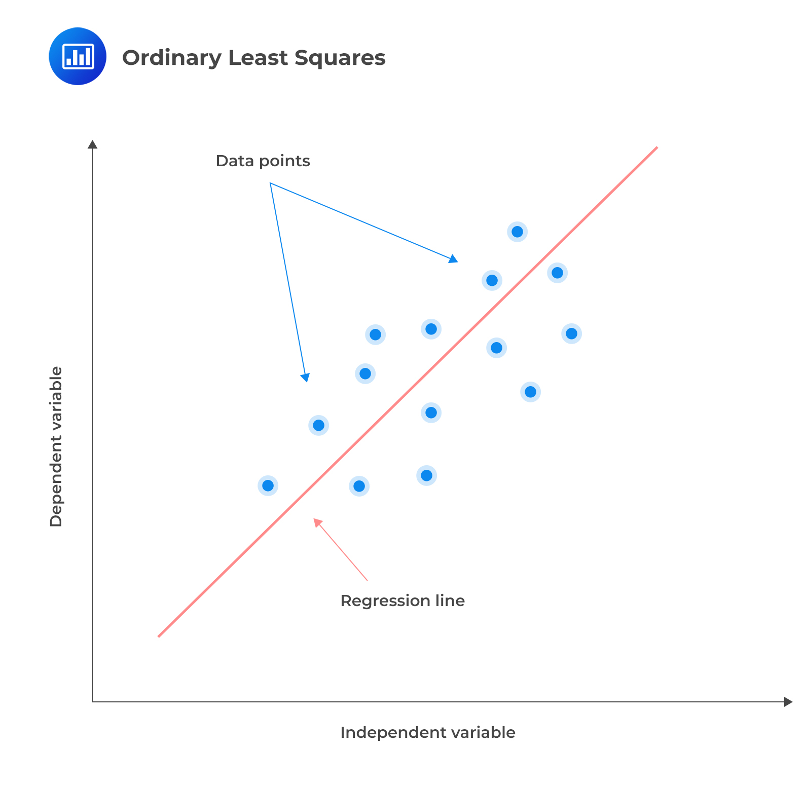The regression line can be expressed as follows:

$$ y =\alpha + \beta_1x_1+ \beta_2x_2 + … + \beta_nx_n $$

Where:

\(y\) = Dependent variable.

\(\alpha\) = Intercept.

\(x_1,x_2,\ldots x_n\) = Independent variables.

\(\beta_1,\beta_2,\ldots,\beta_n\) = Multiple regression coefficients.

The coefficients show the effect of each independent variable on the dependent variable and are calculated based on the data.

The Cost Function for Linear Regression

Training any machine learning model aims to minimize the cost (loss) function. A cost function measures the inaccuracy of the model predictions. It is the sum of squared residuals (RSS) for a linear regression model. This is the sum of the squared difference between the actual and predicted values of the response (dependent variable).

$$ RSS=\sum_{i=1}^{n}\left(y_i-\alpha-\sum_{i=1}^{n}{\beta_jx_{ij}}\right)^2 $$

Where \(x_{ij}\) is the i^th observation and j^th variable.

To measure how well the data fits the line, take the difference between each actual data point \((y)\) and the model’s prediction \((\hat{y})\). The differences are then squared to eliminate negative numbers and penalize larger differences. The squared differences are then added up, and an average is taken.

The advantage of linear regression is that it is easy to understand and interpret. However, it has the following limitations:

• It assumes a linear relationship between the dependent and independent variables.
• It assumes that residuals (the difference between observed and predicted values) are normally distributed and have a constant variance.
• It is prone to overfitting.
• It assumes that there is no multicollinearity.

Example: Prediction Using Linear Regression

Aditya Khun, an investment analyst, wants to predict the return on a stock based on its P/E ratio and the market capitalization of the company using linear regression in machine learning. Khun has access to the P/E ratio and market capitalization dataset for several stocks, along with their corresponding returns. Khun can employ linear regression to model the relationship between the return on a stock and its P/E ratio and market capitalization. The following equation represents the model:

$$ \text{Return} = \beta_0 + \beta_1P/E \text{ ratio} + \beta_2{\text{Market capitalization}} $$

Where:

Return = Dependent variable.

P/E ratio and market capitalization = Independent variables.

\(\beta_0\) = Intercept.

\(\beta_1\) and \(\beta_2\) are the coefficients of the model.

The first step of fitting a linear regression model is estimating the values of the coefficients \(\beta_0\), \(\beta_1\), and \(\beta_2\) using the training data. Coefficients that minimize the sum of the squared residuals are determined.

Suppose we have the following data for 6 stocks:

$$ \begin{array}{c|c|c|c} \textbf{Stock} & \textbf{P/E Ratio} & \textbf{Market cap} & \textbf{Return} \\ & & \bf{(\$ \text{millions})} & \\ \hline 1 & 9 & 200 & 8\% \\ \hline 2 & 11 & 300 & 15\% \\ \hline 3 & 14 & 400 & 18\% \\ \hline 4 & 16 & 500 & 19\% \\ \hline 5 & 18 & 600 & 23\% \\ \hline 6 & 20 & 700 & 27\% \end{array} $$

Given the following parameters and coefficients:

Intercept = 3.432.

P/E Ratio coefficient = −0.114.

Market cap coefficient = 0.0368.

The prediction equation is expressed as follows:

$$ \text{Return} = 3.432 + -0.114\times \text{P\E ratio} + 0.0368\times\text{Market capitalization} $$

Given a P/E ratio of 14 and a market capitalization of $150M, the return of the stock can be determined as follows:

$$ \text{Return} = 3.432 + -0.114\times14 + 0.0368\times150=7.356\% $$

Logistic Regression

When using a linear regression model for binary classification, where the dependent variable Y can only be 0 or 1, the model can predict probabilities outside the range of 0 to 1. This occurs because the model attempts to fit a straight line to the data, and the predicted values may not be restricted to the valid range of probabilities. As a result, the model may produce predictions that are less than zero or greater than one. To avoid this issue, it may be necessary to use a different type of model, such as logistic regression, which is specifically designed for binary classification tasks and ensures that the predicted probabilities are within the valid range. This is achieved by applying a sigmoid function. The sigmoid function graph is shown in the figure below.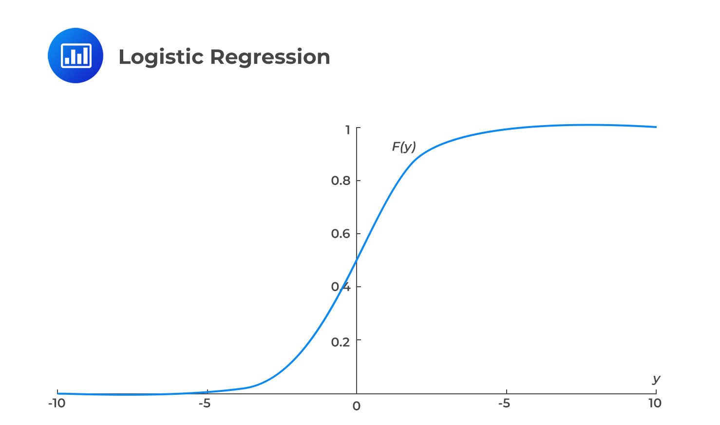

Logistic regression is used to forecast a binary outcome. In other words, it predicts the likelihood of an event occurring based on independent variables, which can be categorical or continuous.

The logistic regression model is expressed as:

$$ F\left(y_j\right)=\frac{e^{y_j} }{1+e^{y_j}} $$

Where:

$$ y_j=\alpha +\beta_1x_{1j} + \beta_{2j}x_{2j}+ … + \beta_{nj}x_{mj} $$

\(\alpha\) = Intercept term.

\(\beta_{ij}\) = Coefficients that must be learned from the training data.

The probability that \(y_j=1\) is expressed as:

$$ p_j=\frac{e^{y_j} }{1+e^{y_j}} $$

$$ \text{Probability that } y_j = 0 \text{ is } (1- p_i) $$

The Cost Function for Logistic Regression

This measures how often we predicted zero when the true answer was one and vice versa. The logistic regression coefficients are trained using techniques such as maximum likelihood estimation (MLE) to predict values close to 0 and 1. MLE works by selecting the values of the model parameters (\(\propto\) and the \(\beta\) s) that maximize the likelihood of the training data occurring. The likelihood function is a mathematical function that describes the probability of the observed data given the model parameters. By maximizing the likelihood function, we can find the values of the parameters most likely to have produced the observed data. This is expressed as:

$$ \prod_{j=1}^{n}{F\left(y_j\right)^{y_j}\left(1-{F(y}_j)\right)^{1-y_j}} $$

Maximizing the log-likelihood function, \(log(L)\), is often easier than the likelihood function itself. The log-likelihood function is obtained by taking the natural logarithm of the likelihood function:

$$ Log\left(L\right)=\sum_{j=1}^{n}\left[y_j\log{\left(F\left(y_j\right)\right)}+\left(1-y_j\right)\log{\left(1-F\left(y_j\right)\right)}\right] $$

Once the model parameters (\(\propto\) and the \(\beta\) s) that maximize the log-likelihood function have been estimated using MLE, predictions can be made using the logistic regression model. To make predictions, a threshold value \(Z\) is chosen. If the predicted probability \(p_j\) is greater than or equal to the threshold \(Z\), the model predicts the positive outcome \((y_j = 1)\); if \(p_j\) is less than the threshold \(Z\), the model predicts a negative outcome \((y_i = 0)\). This is expressed as:

$$ y_j =\left\{\begin{matrix} 1 \text{ if } p_j \ge Z \\ 0 \text{ if } p_j < Z \end{matrix}\right. $$

Example: Using Logistic Regression to Predict Loan Default

A credit analyst wants to predict whether a customer will default on a loan based on their credit score and debt-to-income ratio. He gathers a dataset of 500 customers, with their corresponding credit scores, debt-to-income ratio, and whether they defaulted on the loan. He then splits the data into training and test sets and uses the training data to train a logistic regression model.

The model learns the following relationship between the independent variables (input features) and dependent variables (loan default):

$$ \text{Probability of default} = \frac{e^{\left(-10+\left(0.012 \times \text{Credit score}\right) +\left(0.4 \times \text{Debt-to-income}\right)\right)}}{1 + e^{\left(-10+\left(0.012 \times \text{Credit score}\right) +\left(0.4\times \text{Debt-to-income}\right)\right)}} $$

The above expression calculates the probability that the customer will default on the loan, given their credit score and debt-to-income ratio.

So, if the credit score is 650 and the debt-to-income ratio is 0.6, the probability of default will be calculated as:

$$ \text{Probability of default} = \frac{e^{\left(-10+\left(0.012\times650\right) +\left(0.4 \times0.6\right)\right)}}{1 +\ e^{\left(-10+\left(0.012\times650\right) +\left(0.4 \times0.6\right)\right)}}\approx 12\% $$

So there is a 12% probability that the customer will default on the loan. One can then use a threshold (such as 50%) to convert this probability into a binary prediction (either “default” or “no default”). Since \(12\% < 50\%\), we can classify this as “no default.”

Applications of Logistic Regression

Logistic regression is applied for prediction and classification tasks in machine learning. For example, you could use logistic regression to classify stock returns as either “positive” or “negative” based on a set of input features that you choose. It is simple to implement and interpret. However, it assumes a linear relationship between the dependent and independent variables and requires a large sample size to achieve stable estimates of the coefficients.

Encoding Categorical Variables

Categorical data refers to information presented in groups and can take on values that are names, attributes, or labels. It is not in a numerical format. For example, a given set of stocks can be categorized either as growth or value stocks, depending on the investment style. Many ML algorithms struggle to deal with such data.

It isn’t easy to transform categorical variables, especially non-ordinal categorical data, where the classes are not in any order. Mapping or encoding involves transforming non-numerical information into numbers. One-hot encoding is the most common solution for dealing with non-ordinal categorical data. It involves creating a new dummy variable for each group of the categorical feature and encoding the categories as binary. Each observation is marked as either belonging (Value=1) or not belonging (Value=0) to that group.

Example: One-hot Encoding for Sector, Industry

$$ \begin{array}{c|c|c|c|c|c|c} & \textbf{Utilities} & \textbf{Technology} & \textbf{Transportation} & \textbf{Internet} & \textbf{Airlines} & \textbf{Electric} \\ \hline \text{Meta} & 0 & 1 & 0 & 1 & 0 & 0 \\ \hline \text{Energy} & 1 & 0 & 0 & 0 & 0 & 1 \\ \hline \text{Alibaba} & 0 & 1 & 0 & 1 & 0 & 0 \\ \hline \text{Virgin} & 0 & 0 & 1 & 0 & 1 & 0 \\ \text{Atlantic} & & & & & & \end{array} $$

For ordered categorical variables, for example, where a candidate’s grades are specified as either poor, good, or excellent, a dummy variable that equals 0 for poor, 1 for good, and 2 for excellent can be used.

If an intercept term and correlated dummy variables are included in a model, the dummy variable trap may be encountered. This means that the model will have multiple possible solutions, and we cannot find a unique best-fit solution. To address this issue, techniques such as regularization can be used. These approaches penalize the magnitude of the model’s coefficients, which can help reduce the impact of correlated variables and prevent the dummy variable trap from occurring.

Regularization

Regularization is a technique that prevents overfitting in machine learning models by penalizing large coefficients. It adds a penalty term to the model’s objective function, encouraging the coefficients to take on smaller values. This reduces the impact of correlated variables, as it forces the model to rely more on the overall pattern of the data and less on the influence of any single variable. It improves the generalization of the model to new, unseen data.

Regularization requires the data to be normalized or standardized. Normalization is a method of scaling the data to have a minimum value of 0 and a maximum value of 1. On the other hand, standardization involves scaling the data so that it has a mean of zero and a standard deviation of one. Ridge regression and the least absolute shrinkage and selection operator (LASSO) regression are the two commonly used regularization techniques.

Ridge Regression

Ridge regression, sometimes known as L2 regularization, is a type of linear regression that is used to analyze data and make predictions. It is similar to ordinary least squares regression but includes a penalty term that constrains the size of the model’s coefficients. Consider a dataset with \(n\) observations on each of \(k\) features in addition to a single output variable \(y\) and, for simplicity, assume that we are estimating a standard linear regression model with hats above parameters denoting their estimated values. The relevant objective function (referred to as a loss function) in ridge regression is:

$$ L = \frac{1}{n} \sum_{j=1}^{n}({\widehat{y_j} -\hat{\propto} – \widehat{\beta_1}x_{1j}- \widehat{\beta_2}x_{2j}- \ldots -\widehat{\beta_k}x_{kj})}^2 + \lambda \sum_{i=1}^{k}({\hat{\beta}}_i^2) $$

or

$$ L =\widehat{RSS}+ \lambda \sum_{i=1}^{k}({\hat{\beta}}_i^2) $$

The first term in the expression is the residual sum of squares, which measures how well the model fits the data. The second term is the shrinkage term, which introduces a penalty for large slope parameter values. This is known as regularization, and it helps to prevent overfitting, which is when a model fits the training data too well and performs poorly on new, unseen data.

The parameter \(\lambda\) is a hyperparameter, which means that it is not part of the model itself but is used to determine the model. In this case, it controls the relative weight given to the shrinkage term versus the model fit term. It is essential to tune the value of \(\lambda\), or perform hyperparameter optimization, to find the best value for the given situation. \(\hat{\propto}\) and \(\widehat{\beta_i}\) are the model parameters, while \(\lambda\) is a hyperparameter.

Least Absolute Shrinkage and Selection Operator (LASSO)

LASSO regression, sometimes known as L1 regularization, is similar to ridge regression in that it introduces a penalty term to the objective function to prevent overfitting. However, the penalty term in LASSO regression takes the form of the absolute value of the coefficients rather than the square of the coefficients as in ridge regression.

$$ L = \frac{1}{n} \sum_{j=1}^{n}({\widehat{y_j} – \hat{\propto} – \widehat{\beta_1}x_{1j}- \widehat{\beta_2}x_{2j}- \ldots -\widehat{\beta_k}x_{kj})}^2 + \lambda \sum_{i=1}^{k}{(|\widehat{\beta_i}|}) $$

Also expressed as:

$$ L =\widehat{RSS}+ \lambda \sum_{i=1}^{k}{(|\widehat{\beta_i}|}) $$

In ridge regression, the values of \(\hat{\propto}\) and \(\widehat{\beta_i}\) can be determined analytically using closed-form solutions. This means that the values of the coefficients can be calculated directly, without the need for iterative optimization. On the other hand, LASSO does not have closed-form solutions for the coefficients, so a numerical optimization procedure must be used to determine the values of the parameters.

Ridge regression and LASSO have a crucial difference. Ridge regression adds a penalty term that reduces the magnitude of the \(\beta\) parameters and makes them more stable. The effect of this is to “shrink” the \(\beta\) parameters towards zero, but not all the way to zero. This can be especially useful when there is multicollinearity among the variables, as it can help to prevent one variable from dominating the others.

However, LASSO sets some of the less important \(\beta\) parameters to exactly zero. The effect of this is to perform feature selection, as the \(\beta\) parameters corresponding to the least important features will be set to zero. In contrast, the \(\beta\) parameters corresponding to the more important features will be retained. This can be useful in cases where the number of variables is very large, and some variables are irrelevant or redundant. The choice between LASSO and ridge regression depends on the specific needs of the model and the data at hand.

Elastic Net

Elastic net regularization is a method that combines the L1 and L2 regularization techniques in a single loss function:

$$ L = \frac{1}{n} \sum_{j=1}^{n}({\widehat{y_j} – \hat{\propto} – \widehat{\beta_1}x_{1j}- \widehat{\beta_2}x_{2j}- \ldots -\widehat{\beta_k}x_{kj})}^2 + \lambda_1 \sum_{i=1}^{k}({\hat{\beta}}_i^2)+ \lambda_2 \sum_{i=1}^{k}{(|\widehat{\beta_i}|}) $$

$$ L =\widehat{RSS} + \lambda_1 \sum_{i=1}^{k}({\hat{\beta}}_i^2)+ \lambda_2\ \sum_{i=1}^{k}{(|\widehat{\beta_i}|}) $$

By adjusting \(\lambda_1\) and \(\lambda_2\), which are hyperparameters, it is possible to obtain the advantages of both L1 and L2 regularization. These advantages include decreasing the magnitude of some parameters and eliminating some unimportant ones. This can help to improve the model’s performance and the accuracy of its predictions.

Example: Regularization

$$ \textbf{Table 1: OLS, Ridge and LASSO Regression Estimates} \\ \begin{array}{c|c|c|c|c|c} \textbf{Feature} & \textbf{OLS} & \textbf{Ridge} & \textbf{Ridge} & \textbf{LASSO} & \textbf{LASSO} \\ & & \bf{(\lambda=0.1)} & \bf{(\lambda=0.5)} & \bf{(\lambda =0.01)} & \bf{(\lambda =0.1)} \\ \hline \text{Intercept} & 6.27 & 2.45 & 2.33 & 2.40 & 2.29 \\ \hline 1 & -20.02 & -6.23 & -1.90 & -1.20 & 0 \\ \hline 2 & 51.53 & 9.99 & 2.32 & 1.19 & 0.50 \\ \hline 3 & -32.45 & -2.41 & -0.43 & 0 & 0 \\ \hline 4 & 10.01 & 0.89 & 0.51 & 0 & 0 \\ \hline 5 & -5.92 & -1.64 & -1.22 & -1.01 & 0 \end{array} $$

OLS regression determines the model’s coefficient by minimizing the sum of the squared residuals (RSS). Note that it does not incorporate any regularization and can therefore lead to significant coefficients and overfitting. On the other hand, ridge regularization adds a penalty term to RSS. The penalty term is determined as the sum of the squared coefficient values multiplied by \(\lambda\), which is regarded as a hyperparameter. The hyperparameter controls the strength of the penalty and can be adjusted to find an optimal balance between the model’s fitness and the model’s simplicity. Notice that as \(\lambda\) increases, the penalty term becomes more influential, and the coefficient values become smaller. 

As discussed earlier, LASSO uses the sum of the absolute values of the coefficients as the penalty term. This leads to some coefficients being reduced to zero, eliminating unnecessary model features. Notice the same from the table above. Similar to ridge regression, the strength of the penalty can be modified by adjusting the value of \(\lambda\).

Choosing the value of the hyperparameter in a regularized regression model is an important step in the modeling process, as it can significantly impact the model’s performance. One common approach to selecting the value of the hyperparameter is to use cross-validation, which involves splitting the data into a training set, a validation set, and a test set. This was discussed in detail in Chapter 14. The training fits the model and determines the coefficients for different values of \(\lambda\). The validation set determines how well the model generalizes to new data. The test set is used to evaluate the final performance of the model and provide an unbiased estimate of the model’s accuracy.

Decision Trees

A decision tree is a supervised machine-learning technique that can be used to predict either a categorical target variable, produce a classification tree, or produce a regression tree. It creates a tree-like decision model based on the input features. There is a question at each internal node of the tree, and the algorithm makes a decision based on the value of one of the features. It then branches an observation to another node or a leaf. A leaf is a terminal node that leads to no further nodes. In other words, the decision tree includes the initial root node, decision nodes, and terminal nodes.

Classification and Regression Tree (CART) is a decision tree algorithm commonly used for supervised learning tasks, such as classification and regression. One of the main benefits of CART is that it is highly interpretable, meaning it is easy to understand how the model makes predictions. This is because CART models are built using a series of simple decision rules that are easy to understand and follow. For this reason, CART models are often referred to as “white-box models,” in contrast to other techniques such as neural networks, often referred to as “black-box models.” Neural networks are more challenging to interpret because they are based on complex mathematical equations that are not as easy to understand and follow.

The following is a visual representation of a simple model for predicting whether a company will issue dividends to shareholders based on the company’s profits:

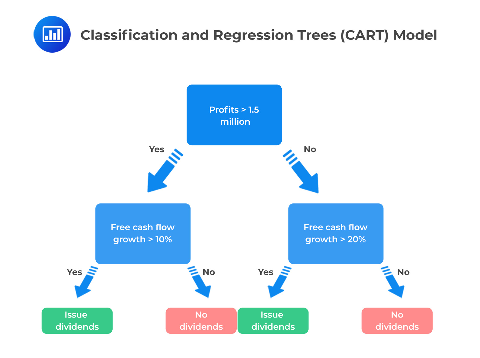
When building a decision tree, the goal is to create a model that can accurately predict the value of a target variable based on the importance of other features in the dataset. To do this, the decision tree must decide which features to split on at each tree node. The tree is constructed by starting at the root node and recursively partitioning the data into smaller and smaller groups based on the values of the chosen features. We use a measure called information gain to determine which feature to split at each node.

Information gain measures how much uncertainty or randomness is reduced by obtaining additional information about the feature. In other words, it measures how much the feature helps us predict the target variable.

There are two commonly used measures of information gain: entropy and the Gini coefficient. Both of these measures are used to evaluate the purity of a node in the decision tree. The goal is to choose the feature that results in the most significant reduction in entropy or the Gini coefficient. This will be the most helpful feature in predicting the target variable.

Entropy ranges from 0 to 1, with 0 representing a completely ordered or predictable system and 1 representing a completely random or unpredictable system. It is expressed as:

$$ \text{Entropy} =-\sum_{i=1}^{K}{p_{i }{log}_{2 }(p_{i })} $$

Where \(K\) is the total number of possible outcomes and \(p_{i}\) the probability of that outcome. The logarithm used in the formula is typically the base-2 logarithm, also known as the binary logarithm.

The Gini measure is expressed as:

$$ \text{Gini} = 1 – \sum_{i=1}^{K}p_i^2 $$

Example: Building a Decision-tree Model to Classify Credit Card Holders as High Risk or Low Risk

A credit card company is building a decision-tree model to classify credit card holders as high-risk or low-risk for defaulting on their payments. They have the following data on whether a credit card holder has defaulted (“Defaulted”) and two features (for the label and the features, in each case, “yes” = 1 and “no” = 0): whether the credit card holder has a high income and whether they have a history of late payments:

$$ \begin{array}{c|c|c} \textbf{Defaulted} & \textbf{High_income} & \textbf{Late_payments} \\ \hline 1 & 1 & 1 \\ \hline 0 & 0 & 0 \\ \hline 0 & 0 & 0 \\ \hline 1 & 1 & 1 \\ \hline 1 & 0 & 1 \\ \hline 0 & 0 & 1 \\ \hline 0 & 1 & 0 \\ \hline 0 & 1 & 0 \end{array} $$

1. Calculate the “Base Entropy” of the Defaulted Series

The base entropy measures the randomness (uncertainty) of the output series before any data is split into separate groups or categories.

$$ \text{Entropy} =-\sum_{i=1}^{K}{p_{i}\log_{2}(p_{i})} $$

Where:

\(K\) = Total number of possible outcomes.

\(p_{i}\) = Probability of that outcome.

The logarithm used in the formula is typically the base-2 logarithm, also known as the binary logarithm.

In this case, three credit card holders defaulted, and five didn’t.

$$ \text{Entropy} =-\left(\frac{3}{8}\log_{2 }\left(\frac{3}{8}\right)+\frac{5}{8}\log_{2}\left(\frac{5}{8}\right) \right)=0.954 $$

2. Build a Decision Tree for This Problem

Both features are binary, so there are no issues with determining a threshold as there would be for a continuous series. The first stage is to calculate the entropy if the split was made for each of the two features. Examining the High_income feature first, among high-income credit card owners (feature = 1), two defaulted while two did not, leading to entropy for this sub-set of:

$$ \text{Entropy}=-\left(\frac{2}{4}\log_{2 }\left(\frac{2}{4}\right)+\frac{2}{4}\log_{2 }\left(\frac{2}{4}\right) \right)=1 $$

Among non-high income credit card owners (feature = 0), one defaulted while three did not, leading to an entropy of:

$$ \text{Entropy}=-\left(\frac{1}{4}\log_{2 }\left(\frac{1}{4}\right)+\frac{3}{4}\log_{2 }\left(\frac{3}{4}\right) \right)=0.811 $$

The weighted entropy for splitting by income level is therefore given by:

$$ \begin{align*} \text{Entropy} &=\frac{4}{8}\times 1+\frac{4}{8}\times0.811=0.906 \\ \\ \text{Information gain} & = 0.954-0.906 = 0.048 \end{align*} $$

We repeat this process by calculating the entropy that would occur if the split was made via the late payment feature.

Three of the four credit card owners who made late payments (feature = 1) defaulted, while one did not.

$$ \text{Entropy}=-\left(\frac{3}{4}\log_{2 }\left(\frac{3}{4}\right)+\frac{1}{4}\log_{2 }\left(\frac{1}{4}\right) \right)=0.811 $$

None of the four credit card owners who did not make late payments (feature = 0) defaulted. The weighted entropy for the late payments feature is, therefore:

$$ \begin{align*} \text{Entropy} & =\frac{4}{8}\times0.811  =0.4055 \\ \\ \text{Information gain} & = 0.954-0.4055 = 0.5485 \end{align*} $$

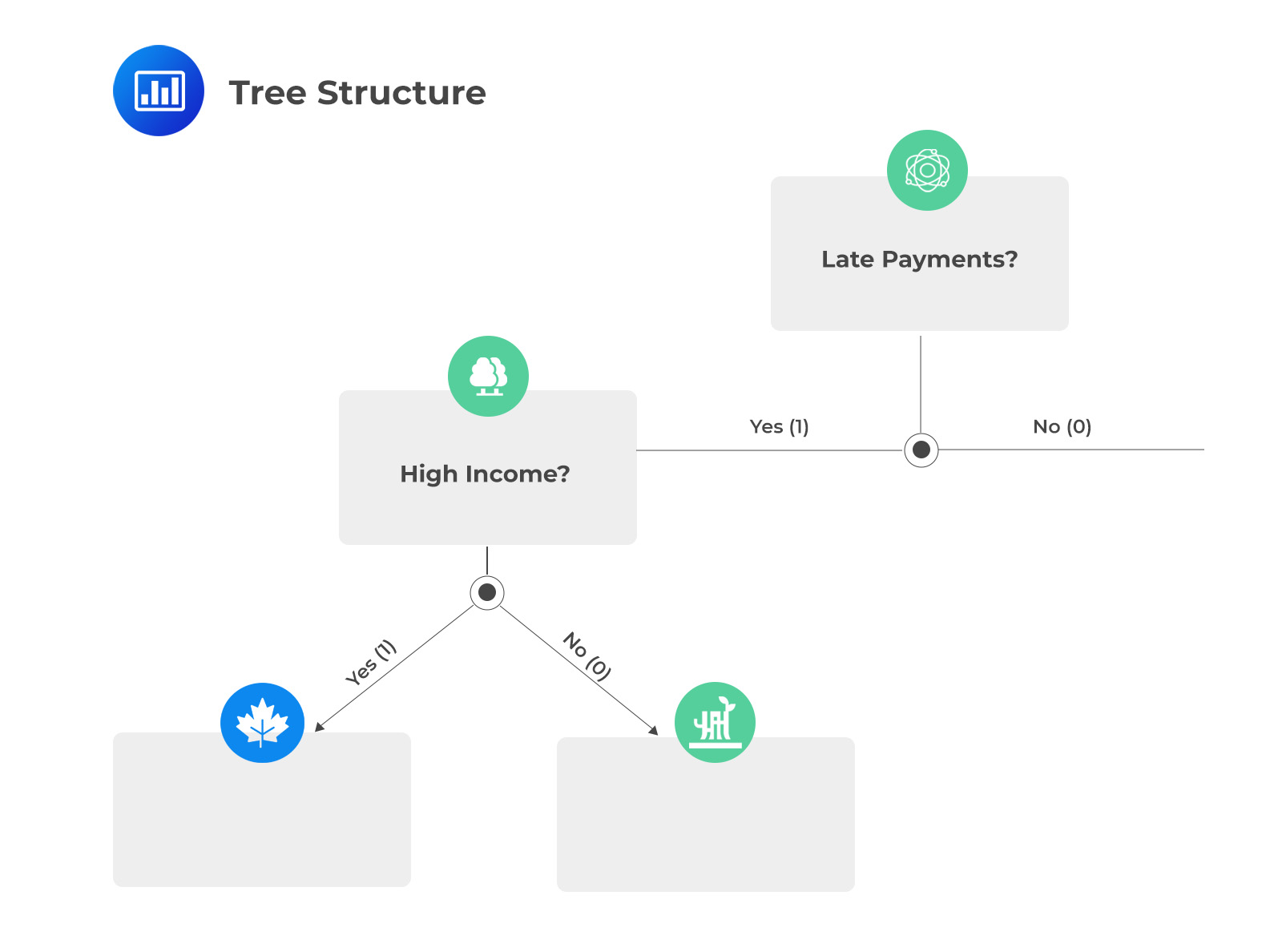
Notice that the entropy is maximized when the sample is first split by the late payments feature. This becomes the root node of the decision tree. For credit card owners who do not make late payments (i.e., the feature =0), there is already a pure split as none of them defaulted. This is to say that credit card holders who make timely payments do not default. This means that no further splits are required along this branch. The (incomplete) tree structure is, therefore:

Ensemble Techniques

Ensemble learning is a machine learning technique in which a group of models, or an ensemble, is used to make predictions rather than relying on the output of a single model. The idea behind ensemble learning is that the individual models in the ensemble may have different error rates and make noisy predictions. Still, by taking the average result of many predictions from various models, the noise can be reduced, and the overall forecast can be more accurate.

There are two objectives of using an ensemble approach in machine learning. First, ensembles can often achieve better performance than individual models (think of the law of large numbers where, as the number of models in the ensemble increases, the overall prediction accuracy tends to improve). Second, ensembles can be more robust and less prone to overfitting, as they are able to average out the errors made by individual models. Some ensemble techniques are discussed below, i.e., bootstrap aggregation, random forests, and boosting.

Bootstrap Aggregation

Bootstrap aggregation, or bagging, is a machine-learning technique that involves creating multiple decision trees by sampling from the original training data. The decision trees are then combined to make a final prediction. A basic bagging algorithm for a decision tree would involve the following steps:

1. Sample the training data with the replacement to obtain multiple subsets of the training data
2. Construct a decision tree on each subset of the training data using the usual techniques.
3. Combine the predictions made by each of the decision tree models, e.g., average, to make a forecast.

Sampling with replacement is a statistical method that involves randomly selecting a sample from a dataset and returning the selected element to the dataset before choosing the next element. This means that an element can be selected multiple times, or it can be left out entirely.

Sampling with replacement allows for the use of out-of-bag (OOB) data for model evaluation. OOB data are observations that were not selected in a particular sample and therefore were not used for model training. These observations can be used to evaluate the model’s performance, as they can provide an estimate of how the model will perform on unseen data.

Random Forests

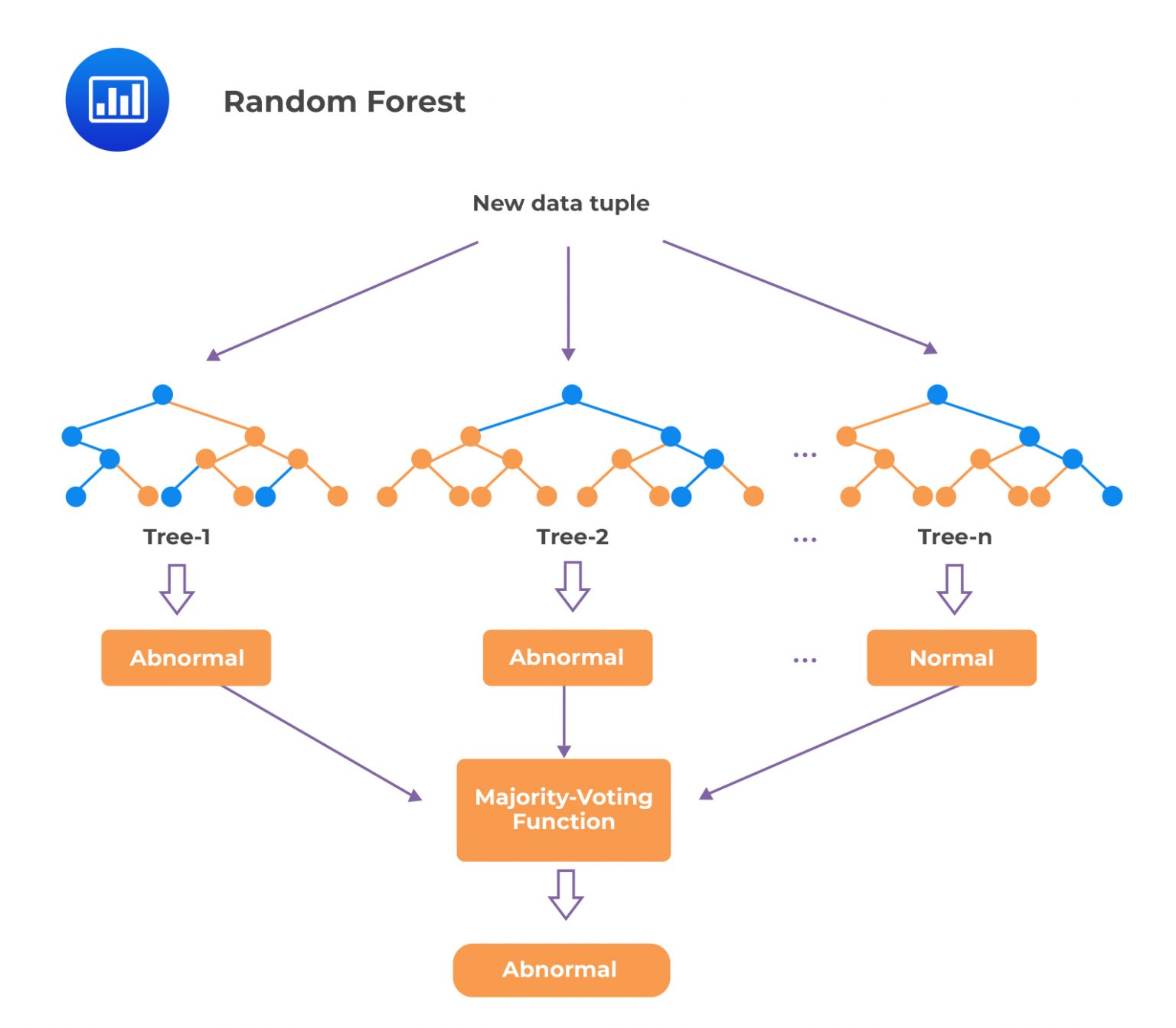
A random forest is an ensemble of decision trees. The number of features chosen for each tree is usually approximately equal to the square root of the total number of features. The individual decision trees in a random forest are trained on different subsets of the data and different subsets of the features, which means that each tree may give a slightly different prediction. However, by combining the predictions of all the trees, the random forest can produce a more accurate final prediction. The performance improvements of ensembles are often greatest when the individual model outputs have low correlations with one another because this helps to improve the model’s generalization.

Boosting

Boosting is an ensemble learning technique that involves training a series of weak models, where each successive model is trained on the errors or residuals of its predecessor. The goal of boosting is to improve the model’s overall performance by combining the weaker models’ predictions to reduce bias and variance. Gradient boosting and AdaBoost (Adaptive Boosting) are the most popular methods.

AdaBoost

AdaBoost is a boosting algorithm that trains a series of weak models, where each successive model focuses more on the examples that were difficult for its predecessor to predict correctly. This results in new predictors that concentrate more and more on the hard cases. Specifically, AdaBoost adjusts the weights of the training examples at each iteration based on the previous model’s performance, focusing the training on the examples that are most difficult to predict. Here is a more detailed description of the process:

1. The AdaBoost algorithm first trains a base classifier (such as a decision tree) on the training data.
2. The algorithm then uses the trained classifier to make predictions on the training set and calculates the errors or residuals between predicted and true labels.
3. The algorithm then adjusts the weights of the training examples based on the previous classifier’s performance, focusing the training on the examples that were most difficult to predict correctly. Specifically, the weights of the misclassified examples are increased, while the weights of the correctly classified examples are decreased.
4. A second classifier is then trained on the updated weights. The whole process is repeated until a predetermined number of classifiers have been trained or until the model’s performance meets a desired threshold.

The final prediction of the AdaBoost model is calculated by combining the predictions of all of the individual classifiers using a weighted sum, where the accuracy of each classifier determines the weights.

Gradient Boosting

In gradient boosting, a new model is trained on the residuals or errors of the previous model, which are used as the target labels for the current model. This process is repeated until a predetermined number of trained models or the model’s performance meets a desired threshold. In contrast to AdaBoost, which adjusts the weights of the training examples at each iteration based on the performance of the previous classifier, gradient boosting tries to fit the new predictor to the residual errors made by the previous predictor.

K-Nearest Neighbors and Support Vector Machine Methods

K-Nearest Neighbors

K-nearest neighbors (KNN) is a supervised machine learning technique commonly used for classification and regression tasks. The idea is to find similarities or “nearness” between a new observation and its k-nearest neighbors in the existing dataset. To do this, the model uses one of the distance metrics described in the previous chapter (Euclidean distance or Manhattan distance) to calculate the distance between the new observation and each observation in the training set. The k observations with the smallest distances are considered the k-nearest neighbors of the new observation. The class label or value of the new observation is determined based on these neighbors’ class labels or values.

KNN is sometimes called a “lazy learner” as it does not learn the relationships between the features and the target like other approaches do. Instead, it simply stores the training data and makes predictions based on the similarity between the new observation and its K-nearest neighbors in the training set.

Here are the basic steps involved in implementing the KNN model:

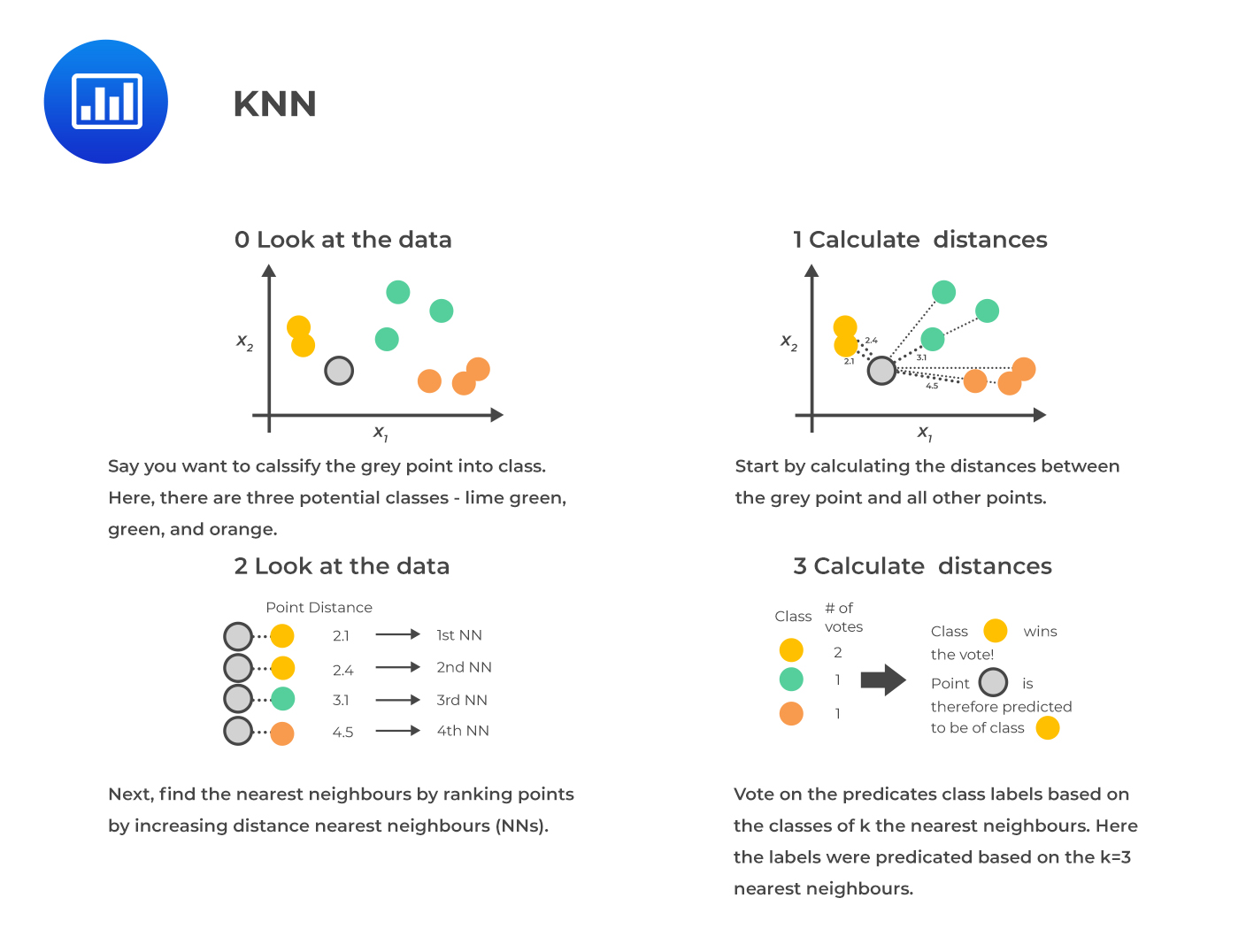Choosing an appropriate value for K is important, as it can impact the model’s ability to generalize to new data and avoid overfitting or underfitting. If K is too large so that many neighbors are selected, it will give a high bias but low variance, and vice versa for small K. If the value of K is set too small, it may result in a more complex model that is more sensitive to individual observations. This may allow the model to fit the training data better. However, it may also make the model more prone to overfitting and not generalize well to new data.

A typical heuristic for selecting K is to set it approximately equal to the square root of the training sample size. For example, if the training sample contains 10,000 points, K could be set to 100 (the square root of 10,000).

Support Vector Machines

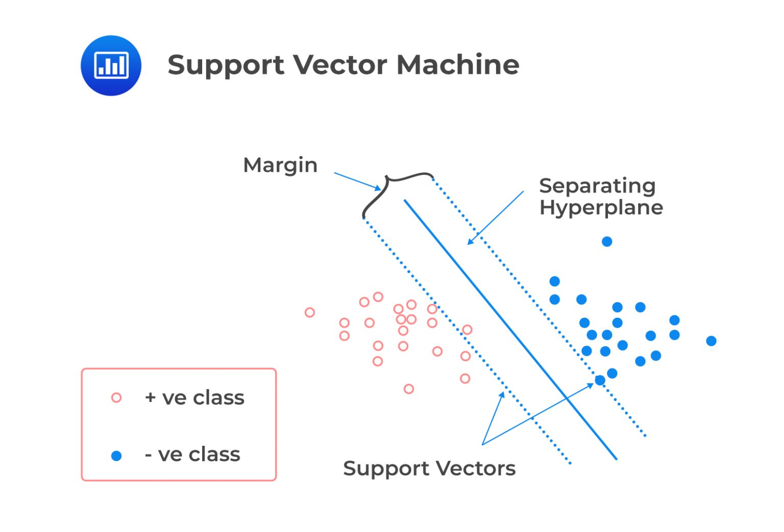
Support vector machines (SVMs) are supervised machine learning models commonly used for classification tasks, particularly when there are many features. SVM works by finding the path’s hyperplane or center that maximizes the distance between the two classes, called the margin.

This hyperplane (the solid blue line in the figure below) is constructed by finding the two parallel lines that are furthest apart and that best separate the observations into the two classes. The data points on the edge of this path, or the points closest to the hyperplane, are called support vectors.

Example: Support Vector Machine

Emma White is a portfolio manager at Delta Investments, a firm that manages diverse investment portfolios for its clients. Delta has a portfolio of “investment-grade” stocks, which are relatively low-risk and have a high likelihood of producing steady returns. The portfolio also includes a selection of “non-investment grade” stocks, which are higher-risk and have the potential for higher returns but also come with a greater risk of loss.

White is considering adding a new stock, ABC Inc., to the portfolio. ABC is a medium-sized company in the retail sector but has not yet been rated by any of the major credit rating agencies. To determine whether ABC is suitable for the portfolio, White decides to use machine learning methods to predict the stock’s risk level. How can Emma use the SVM algorithm to explore the implied credit rating of ABC?

Solution

White would first gather data on the features and target of bonds from companies rated as either investment grade or non-investment grade. She would then use this data to train the SVM algorithm to identify the optimal hyperplane that separates the two classes. Once the SVM model is trained, White can use it to predict the rating of ABC Inc’s bonds by inputting the features of the bonds into the model and noting on which side of the margin the data point lies. If the data point lies on the side of the margin associated with the investment grade class, then the SVM model would predict that ABC Inc’s bonds are likely to be investment grade. If the data point lies on the side of the margin associated with the non-investment grade class, then the SVM model would predict that ABC Inc’s bonds are likely to be non-investment grade.

Neural Networks

Neural networks (NNs), also known as artificial neural networks (ANNs), are machine learning algorithms capable of learning and adapting to complex nonlinear relationships between input and output data. They can be used for both classification and regression tasks in supervised learning, as well as for reinforcement learning tasks that do not require human-labeled training data. A feed-forward neural network with backpropagation is a type of artificial neural network that updates its weights and biases through an iteration process called backpropagation.

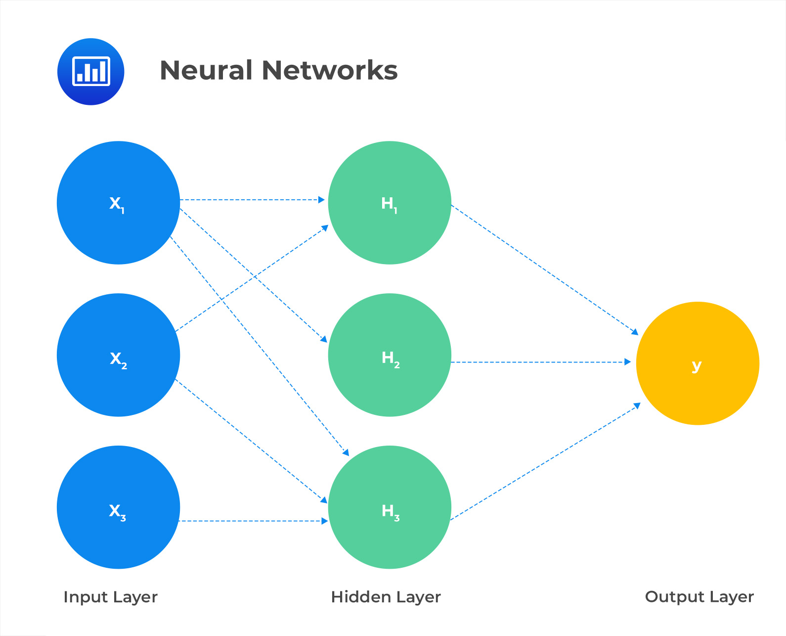In this neural network, there are three input variables, a single hidden layer comprising three nodes and a single output variable. The output variable is determined based on the values of the hidden nodes, which are calculated from the input variables. The equations that are used to determine the values at the hidden nodes are:

$$ \begin{align*} H_1 & = \emptyset(W_{111}X_1 + W_{112}X_2 + W_{113}X_3 + W_1) \\ H_2 & = \emptyset(W_{121}X_1 + W_{122}X_2 + W_{123}X_3 + W_2) \\ H_3 & = \emptyset(W_{131}X_1 + W_{132}X_2 + W_{133}X_3 + W_3) \end{align*} $$

\(\emptyset\) is known as an activation function, which is a nonlinear function that is applied to the linear combination of the input feature values to introduce nonlinearity into the model.  

The value of \(y\) is determined by applying an activation function to a linear combination of the values in the hidden layer.

$$ y = \emptyset (W_{211}H_1 + W_{221}H_2 + W_{231}H_3 + W_4) $$

Where \(W_1\), \(W_2\), \(W_3\), \(W_4\) are biases.

The other \(W\) parameters (coefficients in the linear functions) are weights. As previously stated, if the activation functions were not included, the model would only be able to output linear combinations of the inputs and hidden layer values, limiting its ability to identify complex nonlinear relationships. This is not desirable, as the main purpose of using a neural network is to identify and model these kinds of relationships.

The parameters of a neural network are chosen based on the training data, similar to how the parameters are chosen in linear or logistic regression. To predict the value of a continuous variable, we can select the parameters that minimize the mean squared errors. We can use a maximum likelihood criterion to choose the parameters for classification tasks.

There are no exact formulas for finding the optimal values for the parameters in a neural network. Instead, a gradient descent algorithm is used to find values that minimize the error for the training set. This involves starting with initial values for the parameters and iteratively adjusting them in the direction that reduces the error of the objective function. This process is similar to stepping down a valley, with each step following the steepest descent.

The learning rate is a hyperparameter that determines the size of the step taken during the gradient descent algorithm. If the learning rate is too small, it will take longer to reach the optimal parameters. Still, if it is too large, the algorithm may oscillate from one side of the valley to another instead of accurately finding the optimal values. A hyperparameter is a value set before the model training process begins and is used to control the model’s behavior. It is not a parameter of the model itself but rather a value used to determine how it will be trained and function.

In the example given earlier, the neural network had 16 parameters (i.e., a total of the weights and the biases). The presence of many hidden layers and nodes in a neural network can lead to too many parameters and the risk of overfitting. To prevent overfitting, calculations are performed on a validation data set while training the model on the training data set. As the gradient descent algorithm progresses through the multi-dimensional valley, the objective function will improve for both data sets.

However, at a certain point, further steps down the valley will begin to degrade the model’s performance on the validation data set while continuing to improve it on the training data set. This indicates that the model is starting to overfit, so the algorithm should be stopped to prevent this from happening.

Predictive Performance of Logistic Regression Models vs. Neural Network Models Using a Confusion Matrix

A confusion matrix is a tool used to evaluate the performance of a binary classification model, where the output variable is a binary categorical variable with two possible values (such as “default” or “not default”). It is a 2×2 table that shows the possible outcomes and whether the predicted outcome was correct. A confusion matrix is organized as follows:

$$ \begin{array}{c|c|c} & \textbf{Predicted Positive} & \textbf{Predicted Negative} \\ \hline \text{Actual positive} & TP & FN \\ \hline \text{Actual negative} & FP & TN \end{array} $$

The four elements of the table are:

1. True positive (TP) refers to the number of times the model correctly predicted that a borrower would default on their loan.
2. False negative (FN) refers to the number of times the model incorrectly predicted that a borrower would not default when in fact, they did.
3. False positive (FP) refers to the number of times the model incorrectly predicted that a borrower would default when in fact, they did not.
4. True negative (TN) refers to the number of times the model correctly predicted that a borrower would not default on their loan.

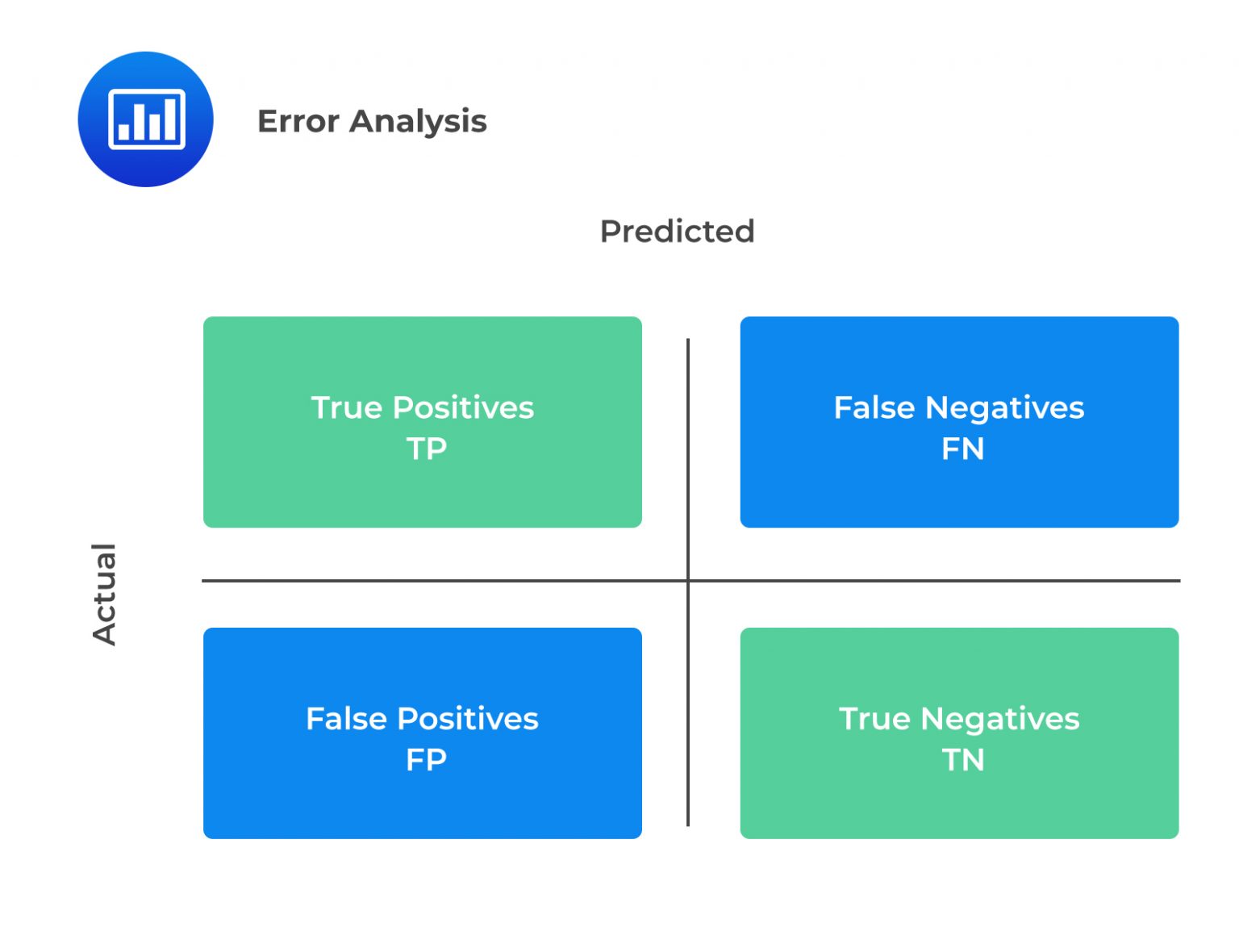The most common performance metrics based on a confusion matrix are:

1. Accuracy: This is the model’s overall accuracy, calculated as the number of correct predictions divided by the total number of predictions. In the case of a binary classification problem, the accuracy is calculated as follows:

   $$ \frac{\left(TP + TN\right)}{\left(TP + TN + FP + FN\right)} $$

2. Precision: This is the proportion of correct positive predictions, calculated as:

   $$ \frac{TP}{\left(TP + FP \right)} $$

3. Recall: This is the proportion of actual positive cases that were correctly predicted, calculated as:

   $$ \frac{TP}{\left(TP + FN \right)} $$

4. The error rate is the proportion of incorrect predictions made by the model, calculated as follows:

   $$ \text{Error rate}=\left(1-\text {Accuracy}\right)\ $$

Example: Confusion Matrix

Suppose we have a dataset of 1600 borrowers, 400 of whom defaulted on their loans and 1200 of whom did not. We can use logistic regression or a neural network to create a prediction model that predicts the likelihood that a borrower will default on their loan. We can set a threshold value to convert the predicted probabilities into binary values of 0 or 1.

Assume that a neural network with one hidden layer and backpropagation is used to model the data. The hidden layer has 5 units, and the activation function used is the logistic function. The loss function used in the optimization process is based on an entropy measure. Note that a loss function is used to evaluate how well a model performs on a given task. The optimization process aims to find the set of model parameters that minimize the loss function. Suppose that the optimization process takes 150 iterations to converge, which means it takes 150 steps to find the set of model parameters that minimize the loss function.

In the context of machine learning, the effectiveness of a model specification is evaluated based on its performance in classifying a validation sample. For simplicity, a threshold of 0.5 is used to determine the predicted class label based on the model’s output probability. If the probability of a default predicted by the model is greater than or equal to 0.5, the predicted class label is “default.” If the probability is less than 0.5, the predicted class label is “no default.”

Adjusting the threshold can affect the true positive and false positive rates in different ways. For example, if the threshold is set too low, the model may have a high true positive rate and a high false positive rate because the model is classifying more observations as positive. On the other hand, if the threshold is set too high, the model may have a low true positive rate and a low false positive rate because the model is classifying fewer observations as positive. This trade-off between true positive and false positive rates is similar to the trade-off between type I and type II errors in hypothesis testing. In hypothesis testing, a type I error occurs when the null hypothesis is rejected when it is actually true. In contrast, a type II error occurs when the null hypothesis is not rejected when it is actually false.

Hypothetical confusion matrices for the logistic and neural network models are presented for both the training and validation samples.

Logistic Regression Training Sample

$$ \begin{array}{c|c|c} & \textbf{Predicted: Default} & \textbf{Predicted: No Default} \\ \hline \text{Actual: Default} & TP = 100 & FN = 300 \\ \hline \text{Actual: No default} & FP = 50 & TN = 1150 \end{array} $$

Logistic Regression Validation Sample

$$ \begin{array}{c|c|c} & \textbf{Predicted: Default} & \textbf{Predicted: No Default} \\ \hline \text{Actual: Default} & TP = 100 & FN = 175 \\ \hline \text{Actual: No default} & FP = 56 & TN = 337 \end{array} $$

Neural Network Training Sample

$$ \begin{array}{c|c|c} & \textbf{Predicted: Default} & \textbf{Predicted: No Default} \\ \hline \text{Actual: Default} & TP = 94 & FN = 306 \\ \hline \text{Actual: No default} & FP = 106 & TN = 1094 \end{array} $$

Neural Network Validation Sample

$$ \begin{array}{c|c|c} & \textbf{Predicted: Default} & \textbf{Predicted: No Default} \\ \hline \text{Actual: Default} & TP = 93 & FN = 182 \\ \hline \text{Actual: No default} & FP = 51 & TN = 342 \end{array} $$

The values in the confusion matrix can be used to calculate various evaluation metrics:

$$ \begin{array}{c|cc|cc} & \textbf{Training} & \textbf{sample} & \textbf{Validation} & \textbf{sample} \\ \hline \textbf{Performance} & \textbf{Logistic} & \textbf{Neural} & \textbf{Logistic} & \textbf{Neural} \\ \textbf{metrics} & \textbf{regression} & \textbf{network} & \textbf{regression} & \textbf{network} \\ \hline \text{Accuracy} & 0.781 & 0.743 & 0.654 & 0.651 \\ \hline \text{Precision} & 0.667 & 0.470 & 0.641 & 0.646 \\ \hline \text{Recall} & 0.250 & 0.235 & 0.364 & 0.338 \end{array} $$

The model appears to perform slightly better on the training data than the validation data, indicating that the model is overfitting. To improve the model’s performance, removing some of the features with limited empirical relevance or applying regularization to the model maybe beneficial. These steps may help reduce overfitting and improve the model’s ability to generalize to new data.

There is not much difference in the performance of the logistic regression and neural network approaches. The logistic regression model has a higher true positive rate but a lower true negative rate for the training data compared to the neural network model. On the other hand, the neural network model appears to have a higher true positive rate but a lower true negative rate for the validation data compared to the logistic regression model.

The Receiver Operating Characteristic Curve

The receiver operating characteristic (ROC) curve is a graphical representation of the trade-off between the true positive rate and the false positive rate, which is illustrated in the figure below. It is calculated by varying the threshold value or decision boundary, classifying predictions as positive or negative, and plotting the true positive rate and the false positive rate at each threshold.

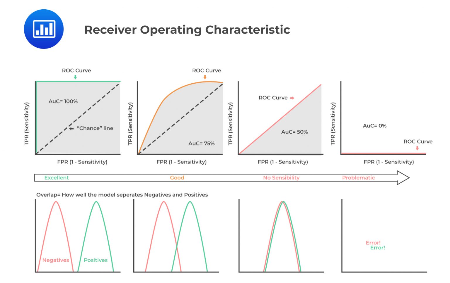A higher area under the receiver operating curve (or area under curve/AUC) value indicates better performance, with a perfect model having an AUC of 1. An AUC value of 0.5 corresponds to the dashed line in the figure above and indicates that the model is no better than random guessing. In contrast, an AUC value less than 0.5 indicates that the model has a negative predictive value.

Practice Question

Consider the following confusion matrices.

Model A

$$ \begin{array}{c|c|c} & \textbf{Predicted:} & \textbf{Predicted:} \\ & \textbf{No Default} & \textbf{Default} \\ \hline \text{Actual: No Default} & TN = 100 & FP = 50\\ \hline \text{Actual: default} & FN = 50 & TP = 900 \end{array} $$

Model B

$$ \begin{array}{c|c|c} & \textbf{Predicted:} & \textbf{Predicted:} \\ & \textbf{No Default} & \textbf{Default} \\ \hline \text{Actual: No Default} & TN = 120 & FP = 80\\ \hline \text{Actual: default} & FN = 30 & TP = 870 \end{array} $$

The model that is most likely to have higher accuracy and higher precision, respectively, is:

1. Higher accuracy: Model A, Higher precision: Model B.
2. Higher accuracy: Model B, Higher precision: Model A.
3. Higher accuracy: Model A, Higher precision: Model A.
4. Higher accuracy: Model B, Higher precision: Model B.

Solution

The correct answer is C.

$$ \text{Model accuracy is calculated as } \frac{(TP + TN) }{(TP + TN + FP\ + FN)} $$

$$ \begin{align*} \text{Model A accuracy} & = \frac{900+100}{900+100+50+50}=0.909 \\ \text{Model B accuracy} & = \frac{870+120}{870+120+80+30}=0.900 \end{align*} $$

Model A has a slightly higher accuracy than model B.

Model precision is calculated as follows:

$$ \frac{TP}{(TP + FP )} $$

$$ \begin{align*} \text{Model precision of A} & =\frac{900}{900+50}=0.9474 \\ \text{Model precision for B} & =\frac{870}{870+80}=0.9158 \end{align*} $$

Model A has a higher precision relative to B.