Future Value and Exposure

After completing this reading you should be able to:

• Describe and calculate the following metrics for credit exposure: expected mark-to-market, expected exposure, potential future exposure, expected positive exposure and negative exposure, effective expected positive exposure, and maximum exposure.
• Compare the characterization of credit exposure to VaR methods and describe additional considerations used in the determination of credit exposure.
• Identify factors that affect the calculation of the credit exposure profile and summarize the impact of collateral on exposure.
• Identify typical credit exposure profiles for various derivative contracts and combination profiles.
• Explain how payment frequencies and exercise dates affect the exposure profile of various securities.
• Explain the general impact of aggregation on exposure, and the impact of aggregation on exposure when there is correlation between transaction values.
• Describe the differences between funding exposure and credit exposure.
• Explain the impact of collateralization on exposure and assess the risk associated with the remargining period, threshold, and minimum transfer amount.
• Assess the impact of collateral on counterparty risk and funding, with and without segregation or rehypothecation.

Credit Exposure

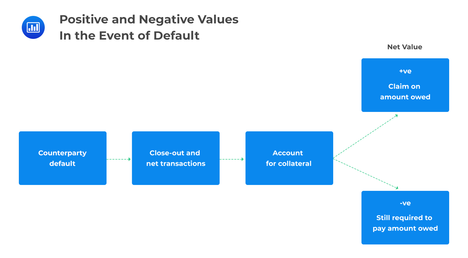
Following an event of default, the surviving counterparty immediately closes out the relevant contracts and all contractual future payments are stopped. The net amount of all the trades, including collateral, held or posted, is determined. This net amount can be positive or negative.

From the perspective of the surviving party, a negative value indicates that the party is in debt to the counterparty and has an obligation to settle the amount. The party cannot just walk away even if the net amount is negative.

From the perspective of the surviving party, a positive value indicates that the party is owed by the counterparty and will have a claim on the positive value at the time of default. As such, the party is in essence an unsecured creditor and will expect to recover some fraction of their claim just as bondholders receive a percentage of the face value of a bond.

Given an event of default, therefore, a party loses if the net value is positive and does not gain if the value is negative.

Metrics for Exposure

Expected Mark-to-market

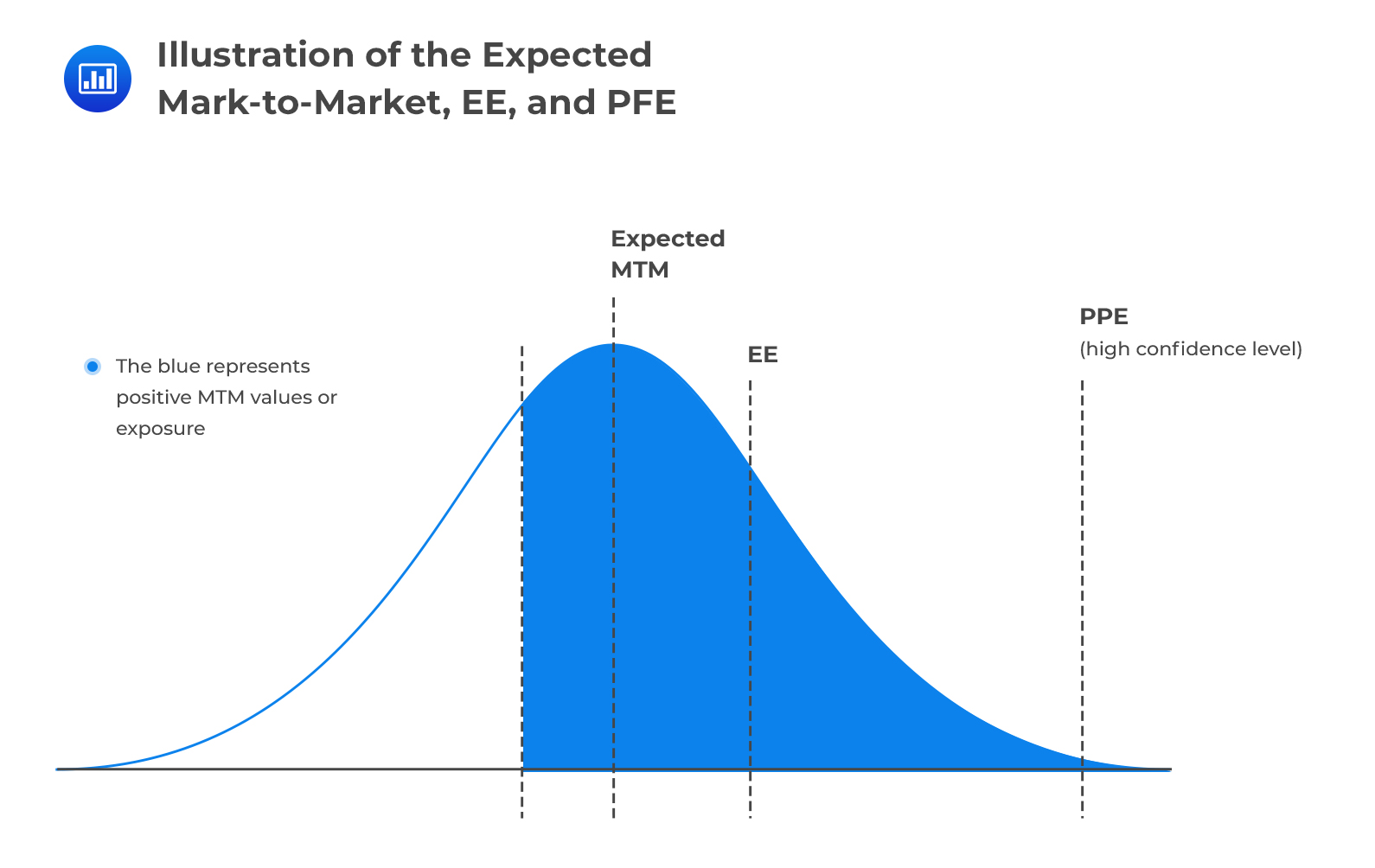
The expected MTM represents the expected (forward) value of a transaction at some point in the future. It can also be interpreted as the average of the future MTM calculated with some probability measure in mind. It takes into account both positive and negative MTM values.

Expected Future Value, EFV

The expected future value, EFV, is the ) is the expected value (forward) of the netted positions at some point in the future. It represents the expected (average) of the future value calculated with some probability measure in mind. It may differ significantly from the current value of the positions.

Expected Exposure, EE

This is the amount expected to be lost if the counterparty defaults when the MTM is positive. It only concerns itself with positive MTM values because they represent situations where the institution would make a loss if the counterparty defaults. By definition, the EE is greater than the expected MTM since it does not take into account negative MTM values.

Example: Expected exposure

Two banks, X and Y, enter into a vanilla interest rate swap with a notional value of $100 million. The banks will exchange payments at six months intervals for the swap’s tenor (5 years).

• Bank X is the floating rate payer and will pay the six-month Libor
• Bank Y is the fixed rate payer and will pay the current swap rate of 5% per annum.

In these circumstances, X and Y both have expected exposure at any future date we may be interested in. For example, Bank X’s 12-month expected exposure is the average market value of the swap to Bank X, 12 months into the future, conditional on positive values.

Why the emphasis on positive values? That’s because a default will hurt Bank X only when the exposure is positive. What’s more, Bank Y’s 12-month expected exposure is the average market value of the swap to Bank Y, 12 months into the future, conditional on positive values.

Potential Future Exposure, PFE

The potential future exposure is the worst exposure an institution could have at a certain time in the future, measured at a specified level of confidence. If the PFE at 95% confidence is X, for example, this implies that we are 95% confident that the maximum possible exposure will be no more than X. Alternatively, X would be exceeded with a probability of no more than 5%.

Using our example above to further illustrate how the PFE is defined, Bank X may have a 12-month PFE of $7.5 million calculated at 99% confidence.

How do we interpret that? It implies that 12 months into the future, the bank is 99% confident that the gain in the swap will be no more than $7.5 million ($7.5m or less), such that a default by the counterparty at the time will expose it to a credit loss of no more than $7.5 million. In other words, the bank is 99% confident that its worst exposure 12 months into the future will be $7.5 million or less.

The PFE is very similar to the traditional measure of value at risk (VaR). The only difference is that:

• While the VaR typically refers to a short horizon, e.g. 10 days, the PFE peers further into the future and can be defined at 3, 4 or 5 years into the future.
• While the VaR refers to the worst-case loss, PFE is normally associated with the worst-case gain (positive exposure)

Note: By definition, the 12-month PFE is greater than the 12-month EE, because the latter is only a mean.

Expected Positive Exposure

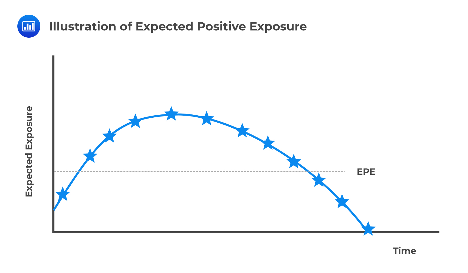
This is the weighted average over time of the expected exposure, EE. The weights are the proportion that an individual EE represents the entire time interval. It is a useful single-number measure of exposure.

Effective Expected Exposure, EEE

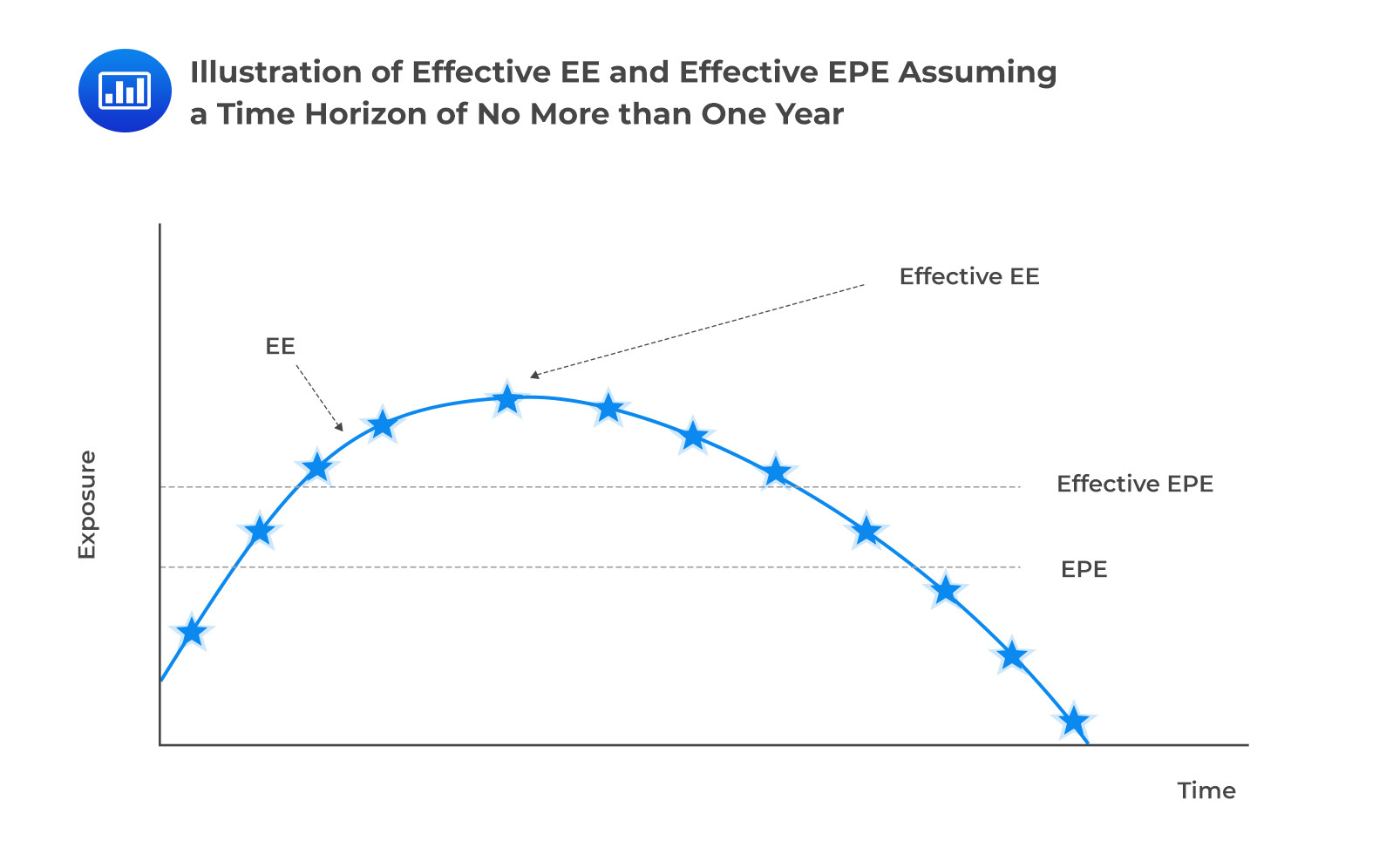
Effective expected exposure is the maximum expected exposure that occurs over the exposure horizon time interval. Effective EE is equal to nondecreasing EE.

Effective EPE, EEPE

Effective expected positive exposure is the weighted average overtime of effective expected exposure.

The effective EPE solves two main problems associated with the EPE:

• Since EPE represents an average of the exposure, it may neglect very large exposures that are present for only a small time.
• EPE may underestimate exposure for short-dated transactions and fail to properly capture “rollover risk”. This applies for current short-dated transactions that will be rolled over into new transactions at their maturity.

Maximum PFE

Maximum PFE simply represents the highest (peak) PFE value over a given time interval.

Negative Exposure

Negative exposure is the exposure from the counterparty’s point of view. It is represented by negative future values.

Negative Expected Exposure, NEE

The negative expected exposure is a mirror image of the EE. To calculate the NEE, all positive MTMs are floored to 0, leaving behind only negative MTMs. NEE tells the financial institution how much the counterparty is exposed to the financial institution.

Expected Negative Exposure, ENE

The expected negative exposure is the exposure owed to the counterparty. It is the mirror image of the expected positive exposure.

Characterization of Credit Exposure to VaR Methods

VaR can be defined as the maximum amount of loss, under normal business conditions, that can be incurred with a given confidence interval. It can also be viewed as the worst possible loss under normal conditions over a specified period.

Suppose an analyst calculates the monthly VaR as $100 million at 95% confidence: What does this imply? It means that under normal conditions, in 95% of the months, we expect the fund to make a profit or lose no more than $100 million. Put differently, the probability of losing $100 million or more in any given month is 5%.

VaR shares several similarities with credit exposure, but there are a few differences:

1. Time horizon: Generally, VaR is defined over a short horizon such as a 10-day period. Exposure on the other hand needs to be defined over many horizons that may stretch several years into the future. By peering into transactions far into the future, exposure involves the analysis of aspects such as future contractual payments, termination events, collateral calls, and exercise decisions. The short-term definition of the VAR implies all these aspects are neglected in its calculation.
2. Risk mitigants: Modeling exposure tends to be more complex compared to value at risk methodologies. Derivative contracts come with risk mitigants that are used to reduce exposure. These include netting agreements, initial margins, and the credit support annex that paves way for posting/return of collateral. All of these mitigants must be modeled, but the process is laden with subjective assumptions. For example, contracts specify a range of eligible collateral securities, and it may not be possible to know with complete certainty the specific type of collateral that will be posted.
3. Application: Whereas VaR is purely a risk management tool, exposure quantification serves both risk management and pricing purposes. This creates additional complexity and can easily lead to two completely different sets of calculations – one for each purpose.

Factors that Affect the Calculation of the Credit Exposure Profile

Future Uncertainty

In contracts where there is a single payout at maturity, uncertainty regarding the value of the final exchange increases over time. For such contracts, exposure is a simple increasing function which follows a “square root of time rule.” That means the exposure is proportional to the square root of time:

$$ \textbf{Exposure} \propto \sqrt { \text{t} } $$

Examples of contracts with a single netted payment include forward rate agreements and FX forwards.

Periodic Cashflows

With contracts that have periodic cash flows, future uncertainty reduces, and therefore the credit exposure is easier to calculate. With an interest rate swap, for example, the expected exposure at the onset of the contract is low. It then increases gradually increases over time before decreasing to zero at maturity.

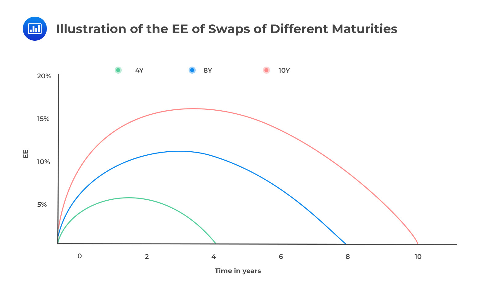Combination of Profiles

When a product is subject to a combination of risk factors, its exposure profile will incorporate all of the underlying risks. An obvious example is a cross-currency swap, which combines an interest rate swap and an FX forward transaction. The contribution of the interest rate swap component to the total exposure is less than that of the FX forward because the latter has considerably higher volatility.

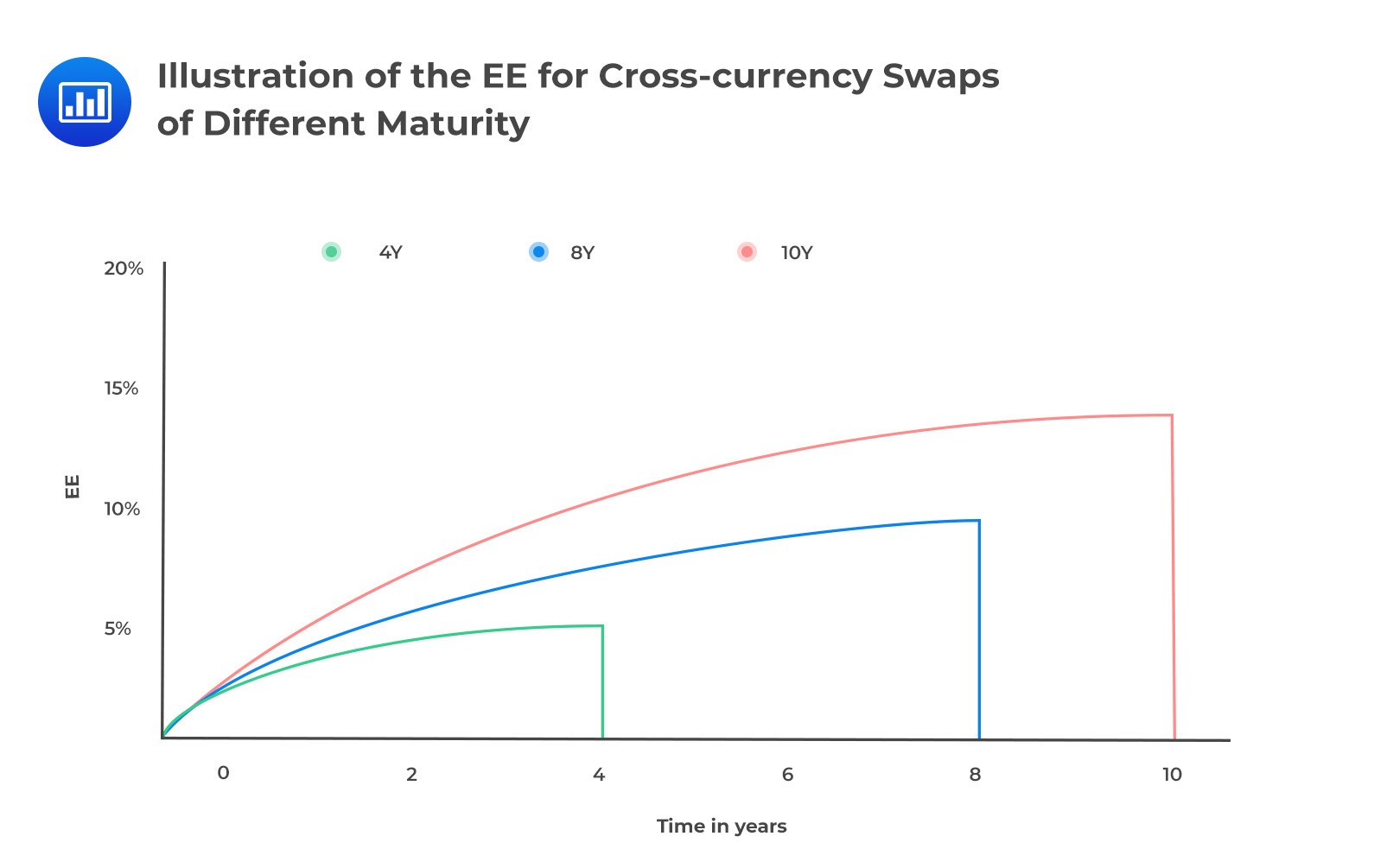Optionality

Exercise decisions create complexity in exposure profiles since after the exercise date (s), the underlying transaction can either cease to exist or continue up to a future date.

Impact of Collateral on Exposure

Collateral typically reduces credit exposure, but that’s only in situations where the exposure is positive because the institution will hold collateral (posted by the counterparty). If the exposure is negative, an institution will be required to post collateral, a situation that will increase the institution’s exposure.

However, collateral doesn’t always remove the risk entirely because of factors such as minimum transfer amounts and delays in receiving collateral.

Example: Impact of collateral on exposure

The table below illustrates the various effects collateral can have on a portfolio. In scenarios 1 and 2, exposure is reduced significantly because collateral is held. Note that the collateral held doesn’t match the exposure because of factors such as sudden increase in MTM, thresholds, and minimum transfer amounts. In scenario 3, the exposure is negative and therefore collateral has to be posted, creating exposure. In scenario 4, the exposure is negative and collateral is posted but this does not increase the exposure (again due to aspects such as thresholds and minimum transfer amounts. Assuming that each scenario has equal weight, the expected exposure can be computed.

$$ \begin{array}{ccc|ccc} \textbf{Future} & \textbf{Value} & {} & \textbf{Total } & \textbf{Exposure} & {} \\ \hline \textbf{Scenario} & {\textbf{No} \\ \textbf{collateral}} & {\textbf{With} \\ \textbf{collateral}} & {\textbf{No} \\ \textbf{collateral}} & {\textbf{With} \\ \textbf{collateral}} & \textbf{Benefit} \\ \hline \text{Scenario 1} & \text{45} & \text{33} & \text{45} & \text{12} & \text{33} \\ \hline \text{Scenario 2} & \text{35} & \text{20} & \text{35} & \text{15} & \text{20} \\ \hline \text{Scenario 3} & \text{-20} & \text{-25} & \text{0} & \text{5} & \text{-5} \\ \hline \text{Scenario 4} & \text{-15} & \text{-13} & \text{0} & \text{0} & \text{0} \\ \hline \text{EE} & \text{} & \text{} & {\frac{80}{4} = 20} & {\frac {32}{4} = 8} & {\frac {48}{4} =12} \\ \end{array} $$

Note: The expected exposure is calculated assuming each scenario has equal weight.

It is also important to note that the treatment of collateral is path-dependent since the amount of collateral required at a given time depends on the amount of collateral called (or posted) in the past. The figure below shows the effect on exposure of three broad cases.

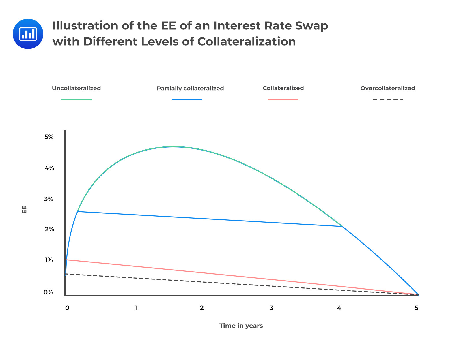Partially collateralized: The reduction of exposure is imperfect due to contractual aspects such as thresholds.

Collateralized: The exposure is reduced significantly since we assume aspects such as thresholds are zero. However, the margin period of risk (MPR) still leads to a reasonably material exposure value.

Overcollateralized: In this case, we further assume that there’s an initial margin and therefore the exposure is significantly reduced. If the initial margin is large enough, the exposure can even be zero.

Typical Credit Exposure Profiles for Various Derivative Contracts

One of the most important determinants of counterparty credit exposure is the time to maturity of the contract. As we peer farther into the future, the uncertainty associated with market variables increases. Let’s now look at the potential future exposure of some securities

Loans, Bonds, and Repos

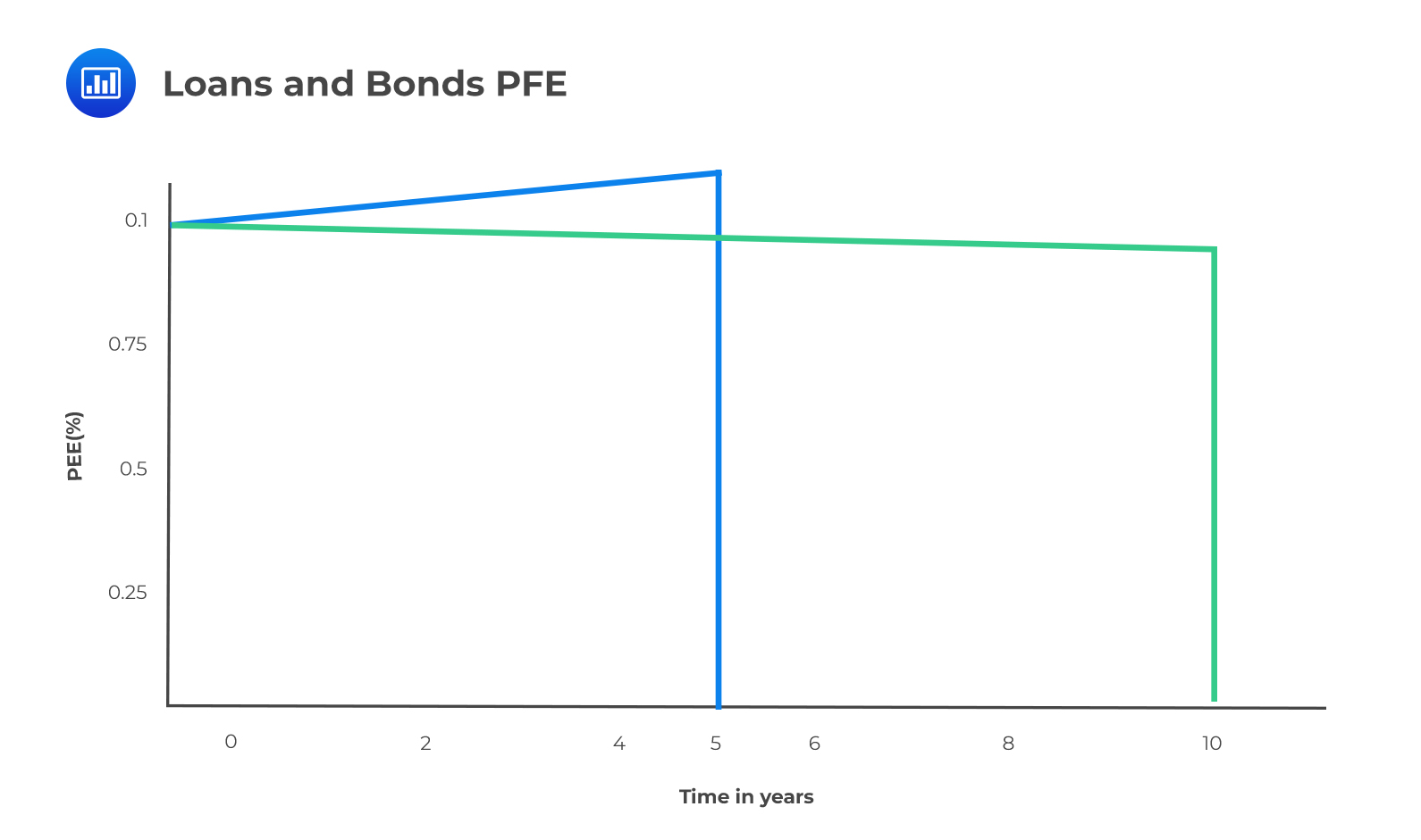
The PFE of bonds, loans, and repos are considered deterministic and are approximately equal to the notional value.

The PFE of loans (from the perspective of the lender), which are typically floating-rate instruments, tends to decrease over time due to the increased probability of prepayments. Bonds, which are typically fixed-rate instruments, tend to have slightly higher exposure than loans of the same maturity because if interest rates decline, the bond may prove less marketable and decrease in price.

Options

The general exposure profile of a long option position is shown in the following figure. Notice that the exposure tends to increase until exercise as a result of the increased possibility that the option can be highly in the money. Although the precise shape of the graph depends on whether the option is in, out, or at the money, the basic shape is the same.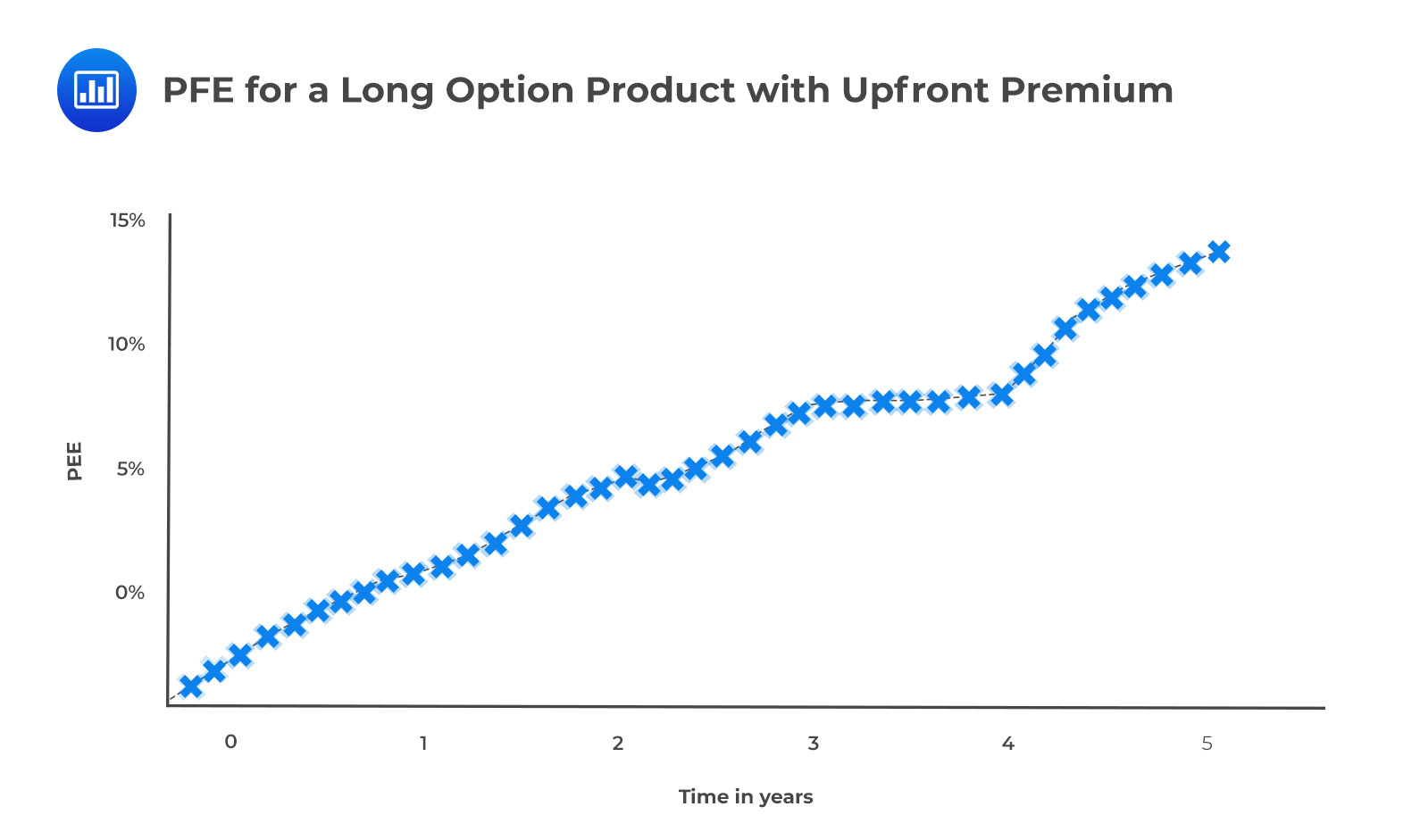

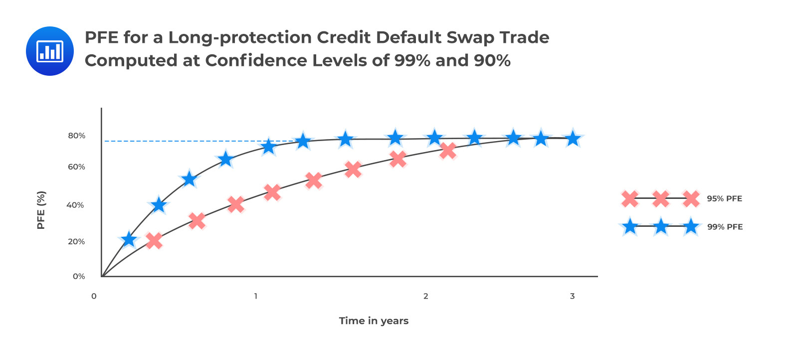
Credit Derivatives

Exposure profiles of credit derivatives are quite difficult to characterize due to (I) wrong-way risk and (II) the discrete payoffs of the instruments. Looking at the exposure profile of a long-protection CDS, we notice that exposure increases in the early stages as a result of the CDS premium (credit spread) widening. The maximum exposure is observed following a credit event which triggers an immediate payment of the notional value less the recovered amount. In our illustrative example below, the exposure is capped at 75%, assuming a 25% recovery value.

Effects of Payment Frequencies and Exercise Dates on the Exposure Profiles of Various Securities

Payment Frequencies

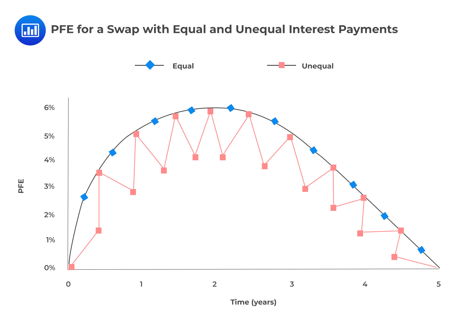
To illustrate the impact of payment frequencies, we will look at interest rate swap PFEs assuming semiannual fixed payments are made while floating quarterly payments are received. As the figure below illustrates, whenever the contract is specified such that there are unequal payments, exposure is reduced when the frequency of receipts is higher than the frequency of payments. The converse is true: exposure is increased when the frequency of payments is higher than the frequency of receipts.

Exercise Dates

The presence of exercise dates makes exposure profiles complex. Let’s look at the exposure of an interest rate swaption that is swap-settled rather than cash-settled (this means there’s physical delivery). The underlying swap also has different payment frequencies. Comparing the swaption with an equivalent forward swap, we find that before the exercise date, the swaption always has a greater exposure than the forward swap. Thereafter, the situation changes, and the forward swap always has a greater exposure than the swaption. The reverse in the trend occurs because there will be scenarios where the forward swap has positive value but the swaption cannot be exercised. The ‘reverse point’ (exercise point) is illustrated in the figure below. There would be an exposure in the forward swap but not the swaption.

Impact of Netting on Exposure

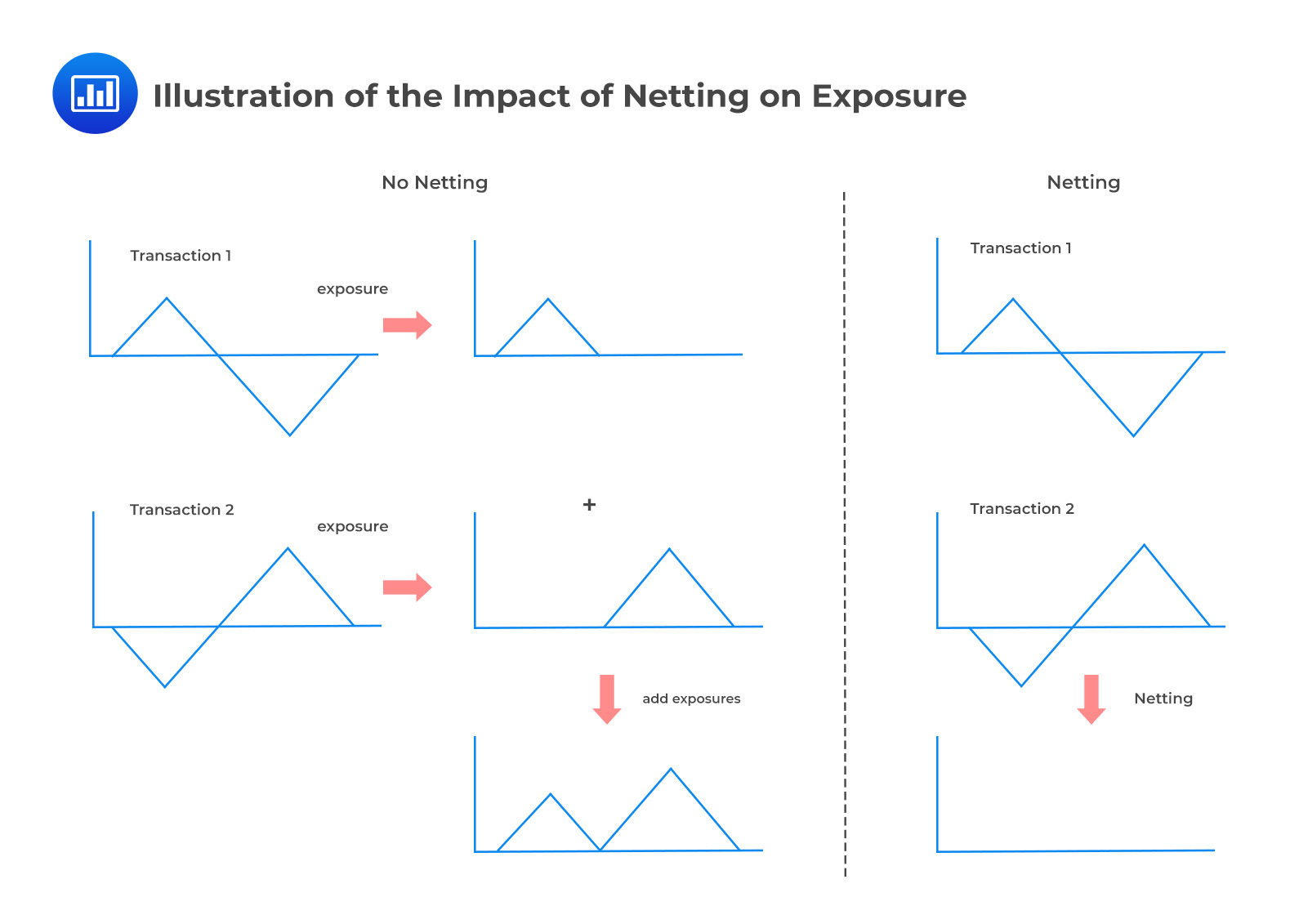
Netting allows two parties to net a set of positions in the event of default of one of them. For netting to occur, however, it must be explicitly covered in the contractual agreement. When netting is not anchored in law, then exposures are considered additive, and positions do not offset one another. Crucially, netting benefits only arise in scenarios where the MTM values of two trades are of opposite signs.

Even more important is the fact that exposure metrics (such as EE) cannot be added to incorporate the impact of netting. Rather, netting must be incorporated before calculating quantities such as EE. The figure below illustrates how two opposite transactions give rise to zero exposure with netting.

Netting and Correlation

When considering the possible netting benefit given a set of transactions, we must consider the correlation between future values. A high positive correlation implies that future values are more likely to be of the same sign, which means there is likely to be very little netting benefit. The netting benefit is lowest when the correlation is 100% (perfect positive correlation). But if the correlation is negative, future values are likely to take on different signs, which means there is likely to be a relatively strong netting benefit. The netting benefit is highest when the correlation is -100% (perfect negative correlation). Te figures below illustrate netting with positive correlation and negative correlation, respectively. In each case, the expected exposure is shown assuming each scenario has equal weight.

$$ \textbf{Netting with Positive Correlation} $$

$$ \begin{array}{ccc|ccc} \textbf{Future} & \textbf{Value} & {} & \textbf{Total} & \textbf{Exposure} & {} \\ \hline \textbf{Scenario} & \textbf{Trade 1} & \textbf{Trade 2} & \textbf{No Netting} & \textbf{Netting} & \textbf{Netting Benefit} \\ \hline \text{Scenario 1} & \text{45} & \text{20} & \text{65} & \text{65} & \text{0} \\ \hline \text{Scenario 2} & \text{25} & \text{15} & \text{40} & \text{40} & \text{0} \\ \hline \text{Scenario 3} & \text{-20} & \text{-25} & \text{0} & \text{0} & \text{0} \\ \hline \text{Scenario 4} & \text{-15} & \text{-10} & \text{0} & \text{0} & \text{0} \\ \hline \text{Scenario 5} & \text{-5} & \text{5} & \text{0} & \text{5} & \text{0} \\ \hline \text{EE} & \text{} & \text{} & \text{22} & \text{21} & \text{1} \\ \end{array} $$

$$ \textbf{Netting with Negative Correlation} $$

$$ \begin{array}{ccc|ccc} \textbf{Future} & \textbf{Value} & {} & \textbf{Total} & \textbf{Exposure} & {} \\ \hline \textbf{Scenario} & \textbf{Trade 1} & \textbf{Trade 2} & \textbf{No Netting} & \textbf{Netting} & \textbf{Netting Benefit} \\ \hline \text{Scenario 1} & \text{45} & \text{-20} & \text{45} & \text{25} & \text{20} \\ \hline \text{Scenario 2} & \text{25} & \text{-15} & \text{25} & \text{10} & \text{15} \\ \hline \text{Scenario 3} & \text{-20} & \text{25} & \text{25} & \text{5} & \text{20} \\ \hline \text{Scenario 4} & \text{15} & \text{-10} & \text{15} & \text{5} & \text{10} \\ \hline \text{Scenario 5} & \text{5} & \text{5} & \text{10} & \text{10} & \text{0} \\ \hline \text{EE} & \text{} & \text{} & \text{24} & \text{11} & \text{13} \\ \end{array} $$

As is evident, negative correlations result in a higher netting benefit

Netting Factor

If we assume that future values of all positions follow a multivariate normal distribution, we can derive the following formula for the “netting factor” with respect to exposure.

$$ \text{Netting factor}=\frac {\sqrt{ \text{n}+\text{n}\left( \text{n}-1 \right) \bar { \rho } }}{ \text{n} } $$

where n represents the number of exposures and \(\bar { \rho }\) is the average correlation.

(Note: Make sure to remember this formula, because GARP has been known to test this concept in its practice exams.)

In essence, the netting factor gives the ratio of net to gross exposure. It takes on a value of +100% if there is no netting benefit (i.e. average correlation = 100%) and 0% when the netting benefit is maximum. It can be shown that the netting benefit improves (netting factor declines) as the number of positions (exposures) increases and as the correlation decreases.

Example: Netting factor

Case 1: 10 positions; \(\bar { \rho }=0.8\)

$$ \text{Netting factor}=\frac {\sqrt{ 10+10\left( 10-1 \right) 0.8 }}{ 10 } =0.9055 $$

Case 2: 15 positions; \(\bar { \rho }=0.6\)

$$ \text{Netting factor}=\frac { \sqrt{15+15\left( 15-1 \right) 0.6 }}{ 15 } =0.7916 $$

Case 3: 20 positions; \(\bar { \rho }=0.5\)

$$ \text{Netting factor}=\frac { \sqrt{20+20\left( 20-1 \right) 0.5 }}{ 10 } =0.0.7246 $$

Note that if there’s no correlation, the netting factor formula simplifies to \(\frac {1}{\sqrt n}\).

For example, if we have three independent transactions with zero mean and equal volatility, their netted exposure reduced to 58% of their exposure without netting. For six exposures, the netting factor decreases to 41%.

Also important to bear in mind is the fact that the netting benefit does depend on the initial MTM of transactions. When there’s a trade with a very strong overall negative MTM, there will be a strong netting benefit because it will offset most (if not all) of the positive MTM of other trades under all scenarios. The converse is true: a very positive MTM reduces the netting benefit because it will offset some (if not all) of the negative MTM of other trades.

Impact of Aggregation on Exposure

The general impact of aggregation on exposure is that it can produce a diversification effect and reduce the overall exposure when compared with the sum of the exposures of each individual transaction. The aggregation process involves combining different transactions to offset one another. An example of this is close-out netting, which is a contractual agreement that allows the future values of different transactions to be netted against one another.

General Impact of Aggregation on Exposure:

• When exposure profiles are offsetting (one is positive while the other is negative), their aggregation results in a reduction in the total exposure.
• The Expected Future Value (EFV) is additive across transactions, as it is simply the average of the values.
• Expected Positive Exposure (EPE) and Expected Negative Exposure (ENE) are not additive because they take into account only positive or negative values respectively. The aggregated EPE or ENE will always be smaller in absolute terms compared to the sum of individual components. This is because aggregation can only reduce exposure in scenarios where the values of the transactions are of opposite signs.

Impact of Correlation on Aggregation:

• If there is a high positive correlation between two transactions, it means that their future values are likely to be of the same sign, which results in a small or even zero diversification benefit. In other words, the aggregation reduces exposure only marginally.
• Conversely, if there is a negative correlation between transaction values, this is more beneficial for diversification. With negative correlations, transaction values are more likely to have opposite signs, hence offering a stronger aggregation benefit and a more significant reduction in exposure.

When assessing the impact of aggregation, it’s important to consider the correlation between the future values of the transactions, as this will affect the degree of diversification benefit received through aggregation. Aggregation is particularly important for counterparty-specific quantities like Credit Valuation Adjustment (CVA) and other measures related to funding and capital, such as Funding Valuation Adjustment (FVA) and Capital Valuation Adjustment (KVA). Overall, while aggregation can provide a reduction in risk and exposure, the extent of this benefit is highly influenced by the correlational relationship between the aggregated transactions.

Credit Exposure vs. Funding Exposure

Credit exposure defines the loss in the event of a counterparty defaulting. A positive exposure at the time of default corresponds to a claim on the defaulting counterparty. If a party is owed money and the counterparty defaults, the party will incur a loss.

Funding exposure defines costs related to the funding of a derivative contract. Funding costs come about in several ways:

• A trader may need to provide collateral and proceed to obtain cash from the money market or the treasury department. That cash will be lent to the trader at a cost.
• A trader may be forced to hold cash received from other sources — such as coupons received from an investment in bonds and close-out payments — to hedge uncollateralized derivative positions or even post collateral. Holding cash to perform such operations means the trader loses out on potential investments.
• A contract with a positive MTM has inherent funding costs. A positive MTM represents an asset that, unfortunately, cannot be monetized economically. Unlike a treasury bond, for instance, the positive MTM derivative cannot be repoed in return for cash, and hence it has to be funded like any other asset with an associated cost.

It’s also important to note that we also have funding benefits like we have funding benefits. A negative MTM creates a derivative liability that represents a loss that does not need to be paid immediately and acts rather like a loan, providing a funding benefit.

Funding costs are generally recognized via funding value adjustment (FVA).

The concept of funding costs and benefits has parallels with credit exposure. A positive value is at risk when a counterparty defaults. Yet, it is also the amount that has to be funded when the counterparty does not. A negative exposure is associated with a funding benefit. However, there are some distinct differences between funding exposure and credit exposure. Here are a few:

Close-out

Close-out adjustments are only considered in default scenarios and are therefore relevant only in the definition of credit exposure. Close-out adjustments do not apply when considering funding aspects, which are based on MTM.

Margin period of risk

Margin period of risk refers to the effective time between a counterparty ceasing to post collateral and when the underlying transactions have been closed-out or replaced. It’s defined assuming the default of the counterparty and is therefore only relevant for credit exposure.

Netting

Close-out netting applies in a default scenario, and hence credit exposure is defined at the netting set level. On the other hand, funding applies at the overall portfolio level since MTM for different transactions is additive, and collateral received from one counterparty may be posted to another.

Segregation

Segregation almost always reduces counterparty credit risk, but it doesn’t reduce funding costs (i.e., there’s no funding benefit). In the event of the counterparty defaulting, the trader can hold on to (or take ownership of) the collateral to cover close-out losses, thus reducing counterparty credit risk. However, it also means that collateral cannot be used for other purposes, such as being posted as collateral against a negative MTM in another transaction. Thus, segregation doesn’t help mitigate funding exposure. Even if the trader receives the collateral, there will be express requirements not to use it in any other contract.

To mitigate both counterparty risk and funding exposure, collateral posted has to have the following characteristics:

• Cash that’s not segregated; and
• Securities that can be rehypothecated;

However, it’s important to note that for collateral to mitigate counterparty risk, there has to be no adverse correlation between the collateral and the counterparty’s credit quality, i.e., wrong-way risk. In other words, the value of the collateral should not decrease when the counterparty’s creditworthiness worsens.

Impact of Collateralization on Exposure

Collateralization is a process used in over-the-counter (OTC) derivatives trades to mitigate counterparty credit risk. The following is a summary of the impact of collateralization on exposure:

• When margin is received, it reduces positive exposure and increases negative exposure. Receiving margin essentially mitigates counterparty risk because it provides a cushion against losses that might occur in the event the counterparty fails to meet its obligations.
• Conversely, when margin is posted, it can create counterparty risk to the extent that it not offset by the value of the position.
• Collateralization reduces both Expected Positive Exposure (EPE) and Expected Negative Exposure (ENE), as seen in scenario modeling, where positive exposure is significantly reduced when margin is held.

Risk Associated with Remargining Period, Threshold, and Minimum Transfer Amount

The Risk Associated with the Remargin Period

The remargin period, also known as the margin call frequency, is the period from which a collateral call takes place to when collateral is actually delivered. The margin period is a period of great uncertainty and extreme exposure to the collateral receiver because there’s no telling whether the other party will honor the request. In fact, a prudent trader will assume that the party required to post collateral will default during the remargin period.

To be able to stay ahead of the game and mitigate risk, the prudent trader must come up with an estimate of the remargin period that is neither too long nor too short.

• If too short, there will be unnecessary anxiety and perhaps making of decisions that are not well-thought-out.
• If too long, there will be an increased risk.

The following are the considerations to be taken into account when calculating the number of days of the remargin period:

• Valuation/Margin call: The party must establish how long it takes to compute the current exposure and current market value of collateral because this is what informs the decision whether or not to make a call.

• Receiving Collateral: The party must establish how long it takes the counterparty to process a collateral request – from the point the call is made to the point the collateral is released

• Settlement: Collateral will not be received immediately as there is a settlement period depending on the type of collateral. Whereas collateral posted in cash often settles intra-day, government and corporate bonds can take up to three days.

• Grace period: In the event that the collateral is not received within the expected time after a call has been made, the counterparty may be afforded some more time to honor the request before “officially” being declared in default

• Liquidation/Close-out/Re-hedging: The party must take into consideration the fact that liquidating the collateral received will take some time. Closing-out and rehedging the exposure always takes time.

$$ \begin{align*} \textbf{} & \textbf{Example timeline for the remargin period in a worst case scenario} \\ & \textbf{based on the assumption of a daily margin call} \end{align*} $$

$$ \begin{array}{l|c|c} \textbf{} & {\textbf{OTC Derivatives} \\ {(\textbf{CSA}^{\textbf a})}} & {\textbf{Repo} \\ {(\textbf{GMRA}^{\textbf b})}} \\ \hline \text{Valuation/Margin call} & \text{2 days} & \text{–} \\ \hline \text{Receiving collateral} & \text{1 day} & \text{1 day} \\ \hline \text{Settlement} & \text{2 days} & \text{1 day} \\ \hline \text{Grace period} & \text{3 days} & \text{–} \\ \hline \text{Liquidation/close-out and re-hedge} & \text{2 days} & \text{1 day} \\ \hline \text{Total} & \text{10 days} & \text{3 day} \\ \hline \text{Basel II minimum} & \text{10 days} & \text{5 days} \\ \end{array} $$ 

\( {{}^\text{a} \text{Credit Support Annex}} \)
\( {{}^\text{b} \text{Global Master Repurchase Agreement}} \)

It is important to note that longer remargin periods may apply depending on the collateral agreement, the counterparty in question, and even the management structure of the institution concerned. It is not unusual to find parties being more lenient with each other in order to forge and maintain good relations. Crucially, it is important to take into account delays that are occasioned by collateral disputes. Our example above does not consider disputes.

Additional Parameters that Impact the Effectiveness of Collateral in Reducing Counterparty Risk

Threshold: As long the exposure remains below the threshold, collateral cannot be called. Thus, such an exposure will typically be uncollateralized (unless an amount of collateral is already held that is within the margins of the minimum transfer amount).

Minimum Transfer Amount: A collateral call is made only when the exposure exceeds not just the threshold but also the minimum transfer amount.

Independent Amounts: Any independent amount should be considered and will reduce the uncollateralized exposure.

Rounding: Although this causes a minor impact, the overall effect can be large and noticeable when combined with thresholds and MTAs.

Impact of Collateral on Counterparty Risk and Funding Costs with and without Segregation or Rehypothecation.

Posting collateral does reduce counterparty risk and funding costs, but different types of collateral have different levels of efficacy. In this regard:

• Cash that’s not subject to segregation reduces both counterparty risk and funding costs.

• If cash collateral or any other security cannot be rehypothecated due to segregation, there’s a reduction of counterparty risk but not funding costs because the collateral cannot be re-used.

• Securities that can be rehypothecated reduce both counterparty risk and funding costs on condition that sufficient haircuts are applied.

• Counterparty bonds posted as collateral are good at mitigating funding costs because they can be rehypothecated. However, the bonds do little in the way of mitigating counterparty risk because, in the event of default, the bonds will have become less marketable and less valuable.

Practice Question

Given that the number of exposure is 19 and the average correlation is 0.87, determine the netting factor under the assumption is that the future values follow a multivariate normal distribution.

A. 0.9841

B. 0.9605

C. 0.8233

D. 0.9364

The correct answer is D.

Recall that the netting factor is given by:

$$ \text{Netting factor}=\frac { \sqrt { n+n\left( n-1 \right) \bar { \rho } } }{ n } $$

Where \(n\) is given as 19 and \(\bar { \rho } \) is given as 0.87.

Therefore:

$$ \text{Netting factor}=\frac { \sqrt { 19+19\left( 19-1 \right) \times 0.87 } }{ 19 } =0.9364 $$