


Modeling Cycles: MA, AR, and ARMA Models
After completing this reading you should be able to: Describe the properties of... Read More

After completing this reading, you should be able to:
Besides annual interest payments, most securities on today’s market have much shorter accrual periods. For Example, interest may be payable monthly, quarterly (every three months), or semi-annually resulting in different present values or future values depending on the frequency of compounding employed. Here’s how to calculate the PV and the FV of an investment with multiple compounding periods per year.
The most important thing is to ensure that the interest rate used corresponds to the number of compounding periods present per year.
$$ \text{FV}=\text{PV}{ \left\{ \left( 1+\cfrac { { \text{r} }_{ \text{q} } }{ \text{m} } \right) \right\} }^{ \text{m}\times \text{n} }$$
Where:
\( {\text{r}}_{\text{q}}\) is the quoted annual rate,
m represents the number of compounding periods (per year)
Lastly, n is the number of years
If we make \(PV\) the subject of the formula above, we have:
$$ \text{PV}=\text{FV}{ \left\{ \left( 1+\cfrac { { \text{r} }_{ \text{q} } }{ \text{m} } \right) \right\} }^{ \text{-m}* \text{n}} $$
Suppose you wish to have $20,000 in your savings account at the end of the next four years. Assume that the account offers a return of 10 percent per year, compounded monthly. How much would you need to invest now to have the specified amount after the four years?
First, we write down the formula to use,
$$ \text{PV}=\text{FV}{ \left\{ \left( 1+\cfrac { { \text{r} }_{ \text{q} } }{ \text{m} } \right) \right\} }^{ \text{-m}* \text{n}} $$
Second, we establish the components that we already have:
\( {\text{r}}_{\text{q}}\)=0.10
m=12
n=4 years
Then, we factor everything into the equation to find our PV.
$$ \text{PV}=20000{ \left\{ 1+\cfrac { 0.1 }{ 12 } \right\} }^{ -12\times 4 }=$13,429 $$
Therefore, you will need to invest at least $13,429 in your account to ensure that you have $20,000 after three years.
We can do this with the financial calculator with the following inputs:
$$ \begin{align*} \text{N} & = 12*4 = 48; \frac {\text{I}}{\text{Y}} =\frac {10}{12} = 0.833; \text{PMT} = 0; \text{FV} = 20,000; \\ \text{CPT} & \Rightarrow \text{PV} = -13,429 \end{align*} $$
Here, we can see that the PV on the financial calculator is a negative value since it’s a cash outflow. The FV has a positive sign since it’s a cash inflow.
We can also rearrange the future value formula to obtain the holding period return (HPR) as follows:
$$ { \text{r} }_{ \text{q} }=\text{m}\left[ { \left( \cfrac { \text{FV} }{ \text{PV} } \right) }^{ \frac { 1 }{ \text{mn} } }-1 \right] $$
If we have a series of interest swap rates, it is possible to derive discount factors. The notional amount, which is technically never exchanged between counterparties, determines the size of both fixed and floating leg payments.
If we could exchange the notional amount, the fixed leg of the swap would resemble a fixed coupon-paying bond, with fixed leg payments acting like semi-annual, fixed coupons, and the notional amount acting like the principal payment. Floating rate payments would act like coupon payments of the floating-rate bond.
We denote the discount factor for t-years as d(t). The methodology used to come up with discount factors when dealing with interest rate swaps is similar to that used to find discount factors when dealing with bonds.
Compute the discount factors for maturities ranging from six months to two years, given a notional swap amount of $100 and the following swap rates:
$$ \begin{array}{c|c} \textbf{Maturity (years)} & \textbf{Swap rates} \\ \hline {0.5} & {0.75} \\ \hline {1.0} & {0.85} \\ \hline {1.5} & {0.98} \\ \hline {2.0} & {1.20} \\ \end{array} $$
The four discount factors d(0.5), d(1.0), d(1.5) and d(2.0) can be calculated as follows:
$$ \begin{align*} { \left( 100+\cfrac { 0.75 }{ 2 } \right) }\text{d}\left( 0.5 \right) & =100 \\ d\left( 0.5 \right) & =\cfrac { 100 }{ 100.375 } =0.9963 \end{align*} $$
$$ \dots \dots \dots \dots \dots \dots \dots \dots \dots \dots \dots \dots $$
$$ \begin{align*} \cfrac { 0.85 }{ 2 } \text{d}\left( 0.5 \right) +\left( 100+\cfrac { 0.85 }{ 2 } \right) \text{d}\left( 1.0 \right) & =100 \\ 0.425 \times0.9963+100.425 \text{ d}(1.0) & =100 \\ \text{d}\left( 1.0 \right) =\cfrac { 100-0.4234 }{ 100.425 } & =0.9916 \end{align*} $$
$$ \dots \dots \dots \dots \dots \dots \dots \dots \dots \dots \dots \dots $$
$$ \begin{align*} \cfrac { 0.98 }{ 2 } \text{ d}\left( 0.5 \right) +\cfrac { 0.98 }{ 2 } \text{d}\left( 1.0 \right) +\left( 100+\cfrac { 0.98 }{ 2 } \right) \text{d}\left( 1.5 \right) & =100 \\ 0.49\times0.9963+0.49\times0.9916+100.49 \text{ d}\left( 1.5 \right) & =100 \\ \text{d}\left( 1.5 \right) =\cfrac { 100-0.4882-0.4859 }{ 100.49 } & =0.9854 \end{align*} $$
$$ \dots \dots \dots \dots \dots \dots \dots \dots \dots \dots \dots \dots $$
$$\begin{align*} \cfrac { 1.20 }{ 2 } \text{d}\left( 0.5 \right) +\cfrac { 1.20 }{ 2 } \text{d}\left( 1.0 \right) +\cfrac { 1.20 }{ 2 } \text{d}\left( 1.5 \right) \left( 100+\cfrac { 1.20 }{ 2 } \right) \text{d}\left( 2.0 \right) & =100 \\ \text{d}\left( 2.0 \right) =\cfrac { 100-0.5978-0.5950-0.5912 }{ 100.6 } & =0.9763 \end{align*}$$
$$ \begin{array}{c|c} \textbf{Maturity (years)} & \textbf{Discount factor} \\ \hline {0.5} & {0.9963} \\ \hline {1.0} & {0.9916} \\ \hline {1.5} & {0.9854} \\ \hline {2.0} & {0.9763} \\ \end{array} $$
A t-period spot rate is a yield to maturity on a zero-coupon bond that matures in t years, assuming semi-annual compounding. We denote the t-periodic spot rate as z(t).
Spot rates and discount factors are related as shown in the following formula, assuming semi-annual coupons:
$$ \text{z}\left( \text{t} \right) =2\left[ { \left( \cfrac { 1 }{ \text{d}\left( \text{t} \right) } \right) }^{ \frac { 1 }{ 2\text{t} } }-1 \right] $$
A spot interest rate gives you the price of a financial contract on the spot date. The spot date is the day when the funds involved in a business transaction are transferred between the parties involved. It could be two days after a trade, or even on the same day, we complete the deal. A spot rate of 5% is the agreed-upon market price of the transaction based on current buyer and seller action.
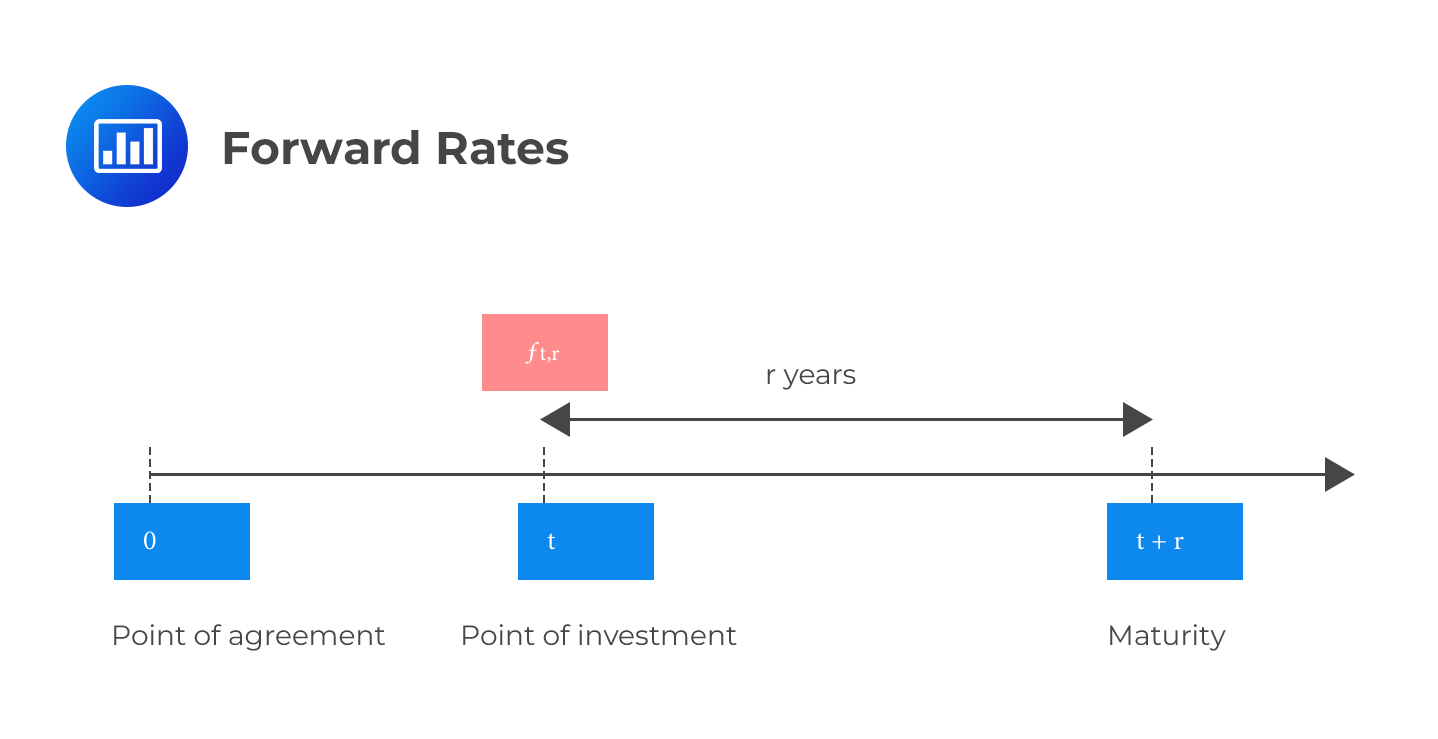
In theory, forward rates are prices of financial transactions that might take place at some future point. The spot rate tells you “how much it would cost to execute a financial transaction today”. The forward rate, on the other hand, tells you “how much would it cost to execute a financial transaction at a future date X”.
We agree on spot and forward rates in the present. The only difference comes in the timing of execution.
 Example: Converting Spot Rates into Forward Rates
Compute the six-month forward rate in six months, given the following spot rates:
Z (0.5) =1.6%
Z (1.0) =2.2%
The six-month forward rate, f(1.0), on an investment that matures in one year, must solve the following equation:
$$ \begin{align*} { \left( 1+\cfrac { 0.022 }{ 2 } \right) }^{ 2 } & ={ \left( 1+\cfrac { 0.016 }{ 2 } \right) }^{ 1 }\times 1+\cfrac { \text{f}{ \left( 1.0 \right) }^{ 1 } }{ 2 } \\ 1.0221 & =1.008\times { \left( 1+\cfrac { \text{f}{ \left( 1.0 \right) } }{ 2 } \right) }^{ 1 } \\ 1.01399-1 & =\cfrac { \text{f}{ \left( 1.0 \right) } }{ 2 } \\ \text{f}\left( 1.0 \right) & =0.02797=2.8\% \end{align*} $$
The par rate is the rate at which the present value of a bond equals its par value. It’s the rate you’d use to discount of all a bond’s cash flows so that the price of the bond is 100 (par). For a 100-par value, the two-year bond that pays semi-annual coupons, and we can easily calculate the 2-year par rate provided we have the discount factor for each period.
$$ \cfrac { \text{Par Rate} }{ 2 }\left[ \text d\left( 0.5 \right) + \text d\left( 1.0 \right) + \text d\left( 1.5 \right) + \text d\left( 2.0 \right) \right] +100 \text{ d}\left( 2.0 \right) =100 … … …(i)$$
In general, for any maturity \(\text{T}\), and assuming a par value of $1,
$$ \cfrac {{ \text{C}}_{\text{T} } }{ 2 } \sum _{ \text{t}=1 }^{ 2\text{T} }{ \text d\left( \cfrac { \text{t} }{ 2 } \right) } + \text{d}\left( \text{T} \right) =1$$
The sum of the discount factors is called the annuity factor, \(\text A_T\), and is given by:
$$ \sum _{ \text{t}=1 }^{ 2\text{T} }{ \text d\left( \cfrac { \text{t} }{ 2 } \right) } $$
Therefore, equation (i) above, becomes
$$ \cfrac { \text{Par Rate} }{ 2 }\left[ A_T \right] +100 \text{ d}\left( T \right) =100$$
Thus,
$$ \text{Par Rate}=\frac{2\times100\times[1-d(T)]}{A_T}$$
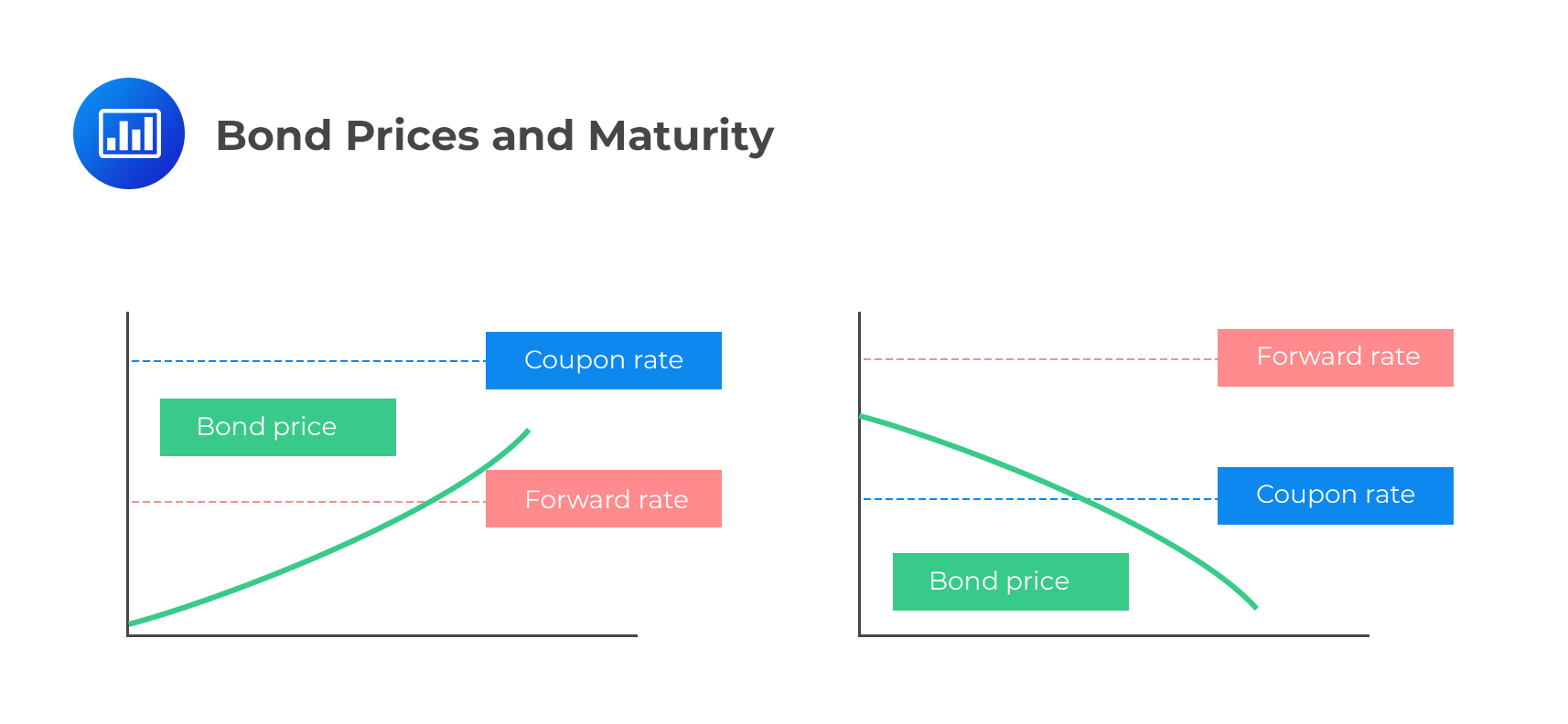
In general terms, bond prices will tend to increase with maturity whenever the coupon rate is above the forward rate throughout the maturity extension. The opposite holds: bond prices will tend to decrease with maturity whenever the coupon rate is below the forward rate for a maturity extension.
 To help you understand just how this happens, assume we have two investors with the opportunity to invest in either STRIPS or a five-year bond. The investor who opts for the 5-year bond (which utilizes forward rates) will have a simple task: they will invest at the onset and then wait to receive regularly scheduled coupon payments, plus the principal amount at maturity. The investor who opts for STRIPS (which utilizes spot rates) will roll them over as they mature throughout the five years. Rolling over implies that when one STRIP expires, the investor will use the proceeds to invest in the next six-month contract, and so on for five years.
In market conditions where short-term rates are above the forward rates utilized by bond prices, the investor who rolls over the STRIPS will tend to outperform the investor in the 5-year bond. The opposite is exact: In market conditions where short-term rates are below the forward rates utilized by bond prices, the investors who roll over the STRIPS will tend to underperform the investor in the 5-year bond.
 Flattening and Steepening of Rate Curves
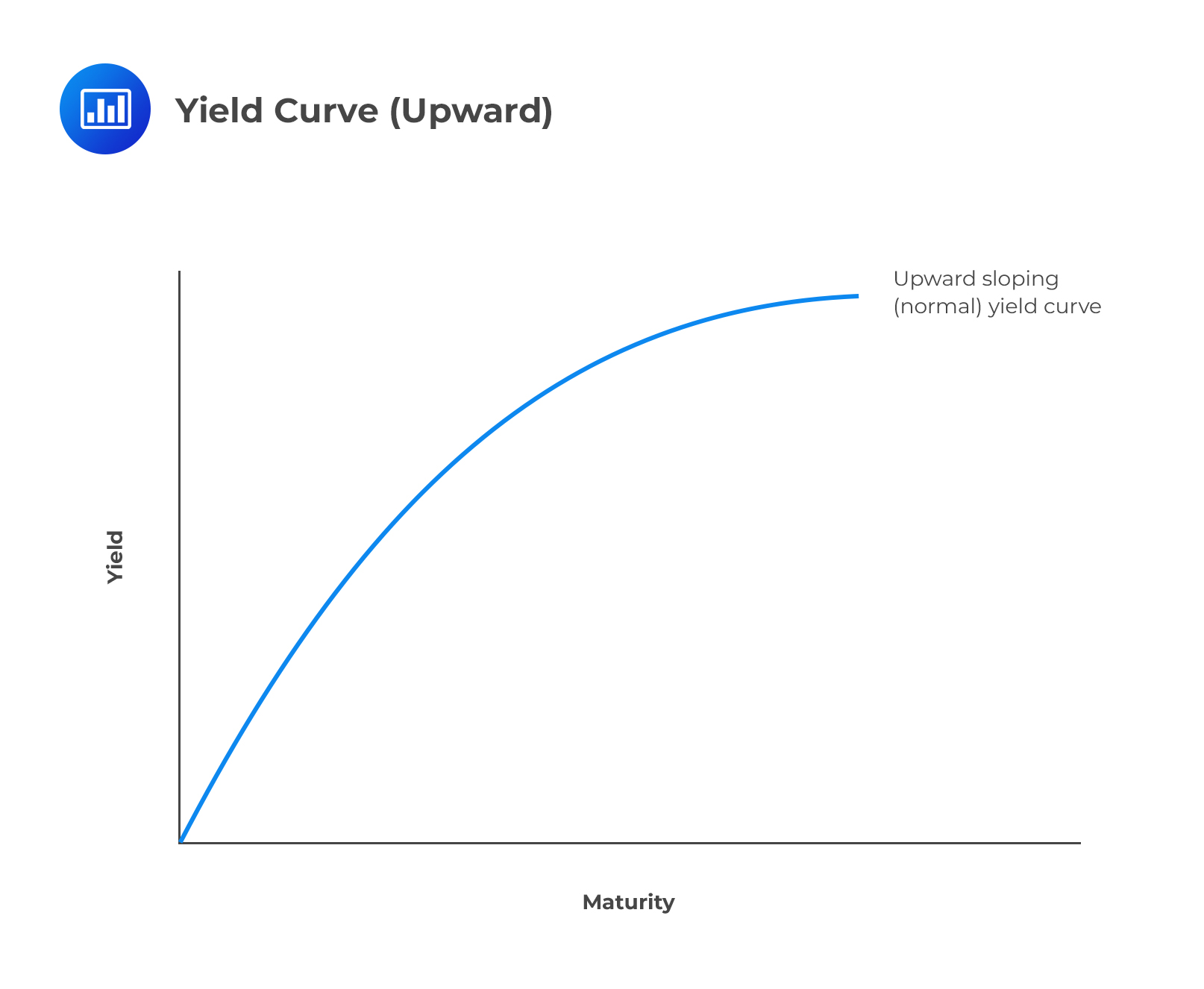
A yield curve represents the yield of each bond along a maturity spectrum that’s plotted on a graph. The most and widely accepted yield curves pit the three-month versus two-year T-bonds or the five-year versus ten-year T-bonds. On occasion, we may use the Federal Funds Rate versus the 10-year Treasury note.
The yield curve typically slopes upwards, indicating that the interest rate on long-term bonds is higher than the rate on short-term bonds, reflecting the investors’ demands to be compensated for taking on more risk by investing in long-term bonds. Such a curve is said to be normal.
 Other than a standard yield curve, we could have a flattening yield curve or a steepening yield curve.
A flat yield curve indicates that little difference exists between short-term and long-term rates for similarly rated bonds. It may manifest as a result of long-term interest rates falling more than short-term interest rates or short-term rates increasing more than long-term rates.
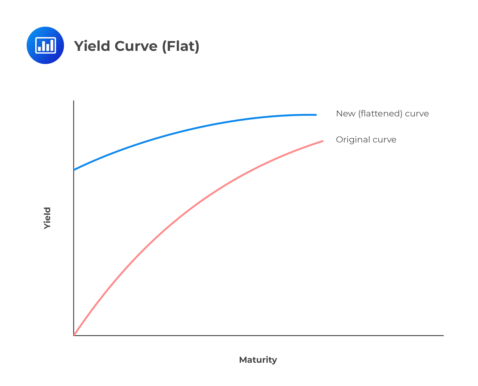 A flattening curve reflects the expectations of investors about the macroeconomic outlook. It may be the result of the following events:
A steepening yield curve indicates a widening gap between the yields on short-term bonds and long-term bonds. A steepening curve could occur when long-term rates rise faster than short-term rates. Sometimes, short-term rates can also show some defiance by decreasing even as long-term rates rise.
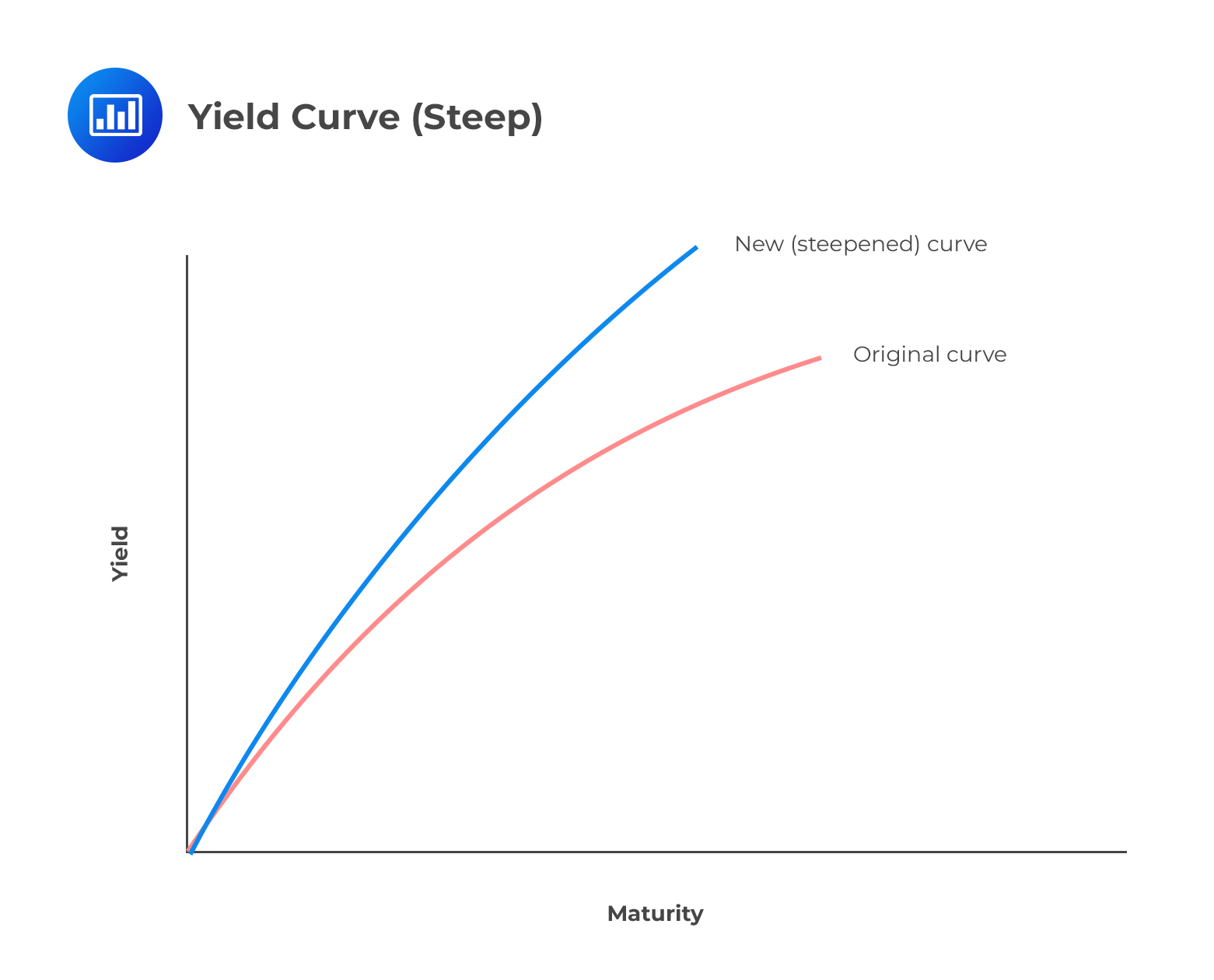 For example, assume that a two-year note was at 2.3% on July 15, and the 10-year was at 3.3%. By August 30, the two-year note could have risen to 2.38% and the 10-year to 3.5%. The difference would effectively go from 1 percentage point to 1.12 percentage points, resulting in a steeper yield curve.
A steepening curve reflects the expectations of investors about the macroeconomic outlook. It may be the result of the following events:
A trader who anticipates a steepening of the yield curve can sell a long-term bond and buy a short-term bond because they expect bond prices to fall in the long-term (bond prices fall as rates increase).
A swap is a financial derivative in which two counterparties agree to exchange streams of payments over time based on specified notional amounts or principal. The parties do not exchange the notional principal but instead agree to swap cash flows derived from it.
In a swap market, the par rate is the fixed interest rate at which the present value of fixed rate payments equals the present value of expected floating rate payments, essentially making the value of the swap zero at initiation.
The par rate reflects a market’s consensus on the equilibrium rate for a standard interest rate swap (market benchmark).
Par rates are computed using the current spot rates for various maturities. The spot rates are implied by the yields on zero-coupon bonds or derived from the yield curve. These rates are then used along with the appropriate discount factors to equate the present values of the fixed and floating payments.
Question 1
Given the following spot rates, compute the 6-month forward rate in 1 year.
\( z\left( 1.0 \right) = 3.25\%\)
\( z\left( 1.5 \right) = 3.60\%\)
A. 4.2%
B. 1.5%
C. 4.3%
D. 5.1%
The correct answer is C.
Solution:
The 6-month forward rate on an investment that matures in 1.5 years must solve the following equation:
$$\begin{align*} { \left( 1+\frac { 0.036 }{ 2 } \right) }^{ 3 }&={ \left( 1+\frac { 0.0325 }{ 2 } \right) }^{ 2 }\times { \left( 1+\frac { f\left( 1.5 \right) }{ 2 } \right) }^{ 1 } \\ 1.05498&=1.03276\times { \left( 1+\frac { f\left( 1.5 \right) }{ 2 } \right) }^{ 1 } \\ 1.02152-1&=\frac { f\left( 1.5 \right) }{ 2 }\\ f\left( 1.5 \right) &=0.04303=4.3\% \end{align*}$$
Question 2
Consider a bond with a par value of USD 1,000 and maturity in four years. The bond pays a coupon of 4% annually. The spot rate curve is as follows:
$$ \begin{array}{l|c} \bf{n} \textbf{-year} & \textbf{Spot rate} \\ \hline 1 & 5\% \\ \hline 2 & 6\% \\ \hline 3 & 7\% \\ \hline 4 & 8\% \\ \hline \end{array} $$
The value of the bond is closest to:
A. $1,160
B. $500
C. $870.78
D. $850
The correct answer is C.
The value of the bond is the present value of all future cash flows (coupons plus principal), discounted at the various spot rates.
$$ \begin{align*} Each \quad coupon=4\% \times 1,000=$40 \\ \end{align*}$$
$$ \begin{align*} PV&=\frac { 40 }{ { \left( 1+0.05 \right) }^{ 1 } } +\frac { 40 }{ { \left( 1+0.06 \right) }^{ 2 } } +\frac { 40 }{ { \left( 1+0.07 \right) }^{ 3 } } +\frac { 40+1000 }{ { \left( 1+0.08 \right) }^{ 4 } } \\ & =38.10+35.60+32.65+764.43=$870.78 \end{align*}$$
Spot, forward, and par rates are core FRM Part I Valuation and Risk Management concepts. Candidates may be tested on yield curve relationships, implied forward rates, bond pricing, and how interest rate movements affect valuation decisions.
Build confidence with the complete FRM Part I prep program featuring guided lessons, question banks, and realistic mock exams.
Access FRM practice questions, study notes, mock exams, and video lessons with AnalystPrep.
Offered by AnalystPrep


Get Ahead on Your Study Prep This Cyber Monday! Save 35% on all CFA® and FRM® Unlimited Packages. Use code CYBERMONDAY at checkout. Offer ends Dec 1st.