Evaluating the Fit of a Machine Learning Algorithm

Model Training

Suppose that the target variable (y) for the ML training model has the sentiment class labels (positive and negative). To ease the calculation of the performance metrics, we relabel them as 1 (for positive) and 0 (for negative). The performance metrics that can be employed here are receiver operating characteristic (ROC) curve and area under the curve (AUC) from the trained model results.

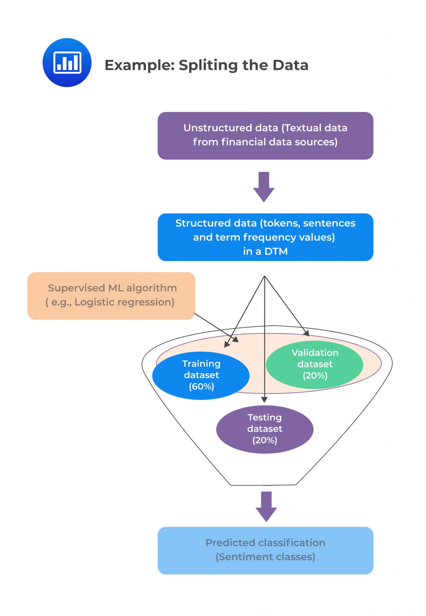
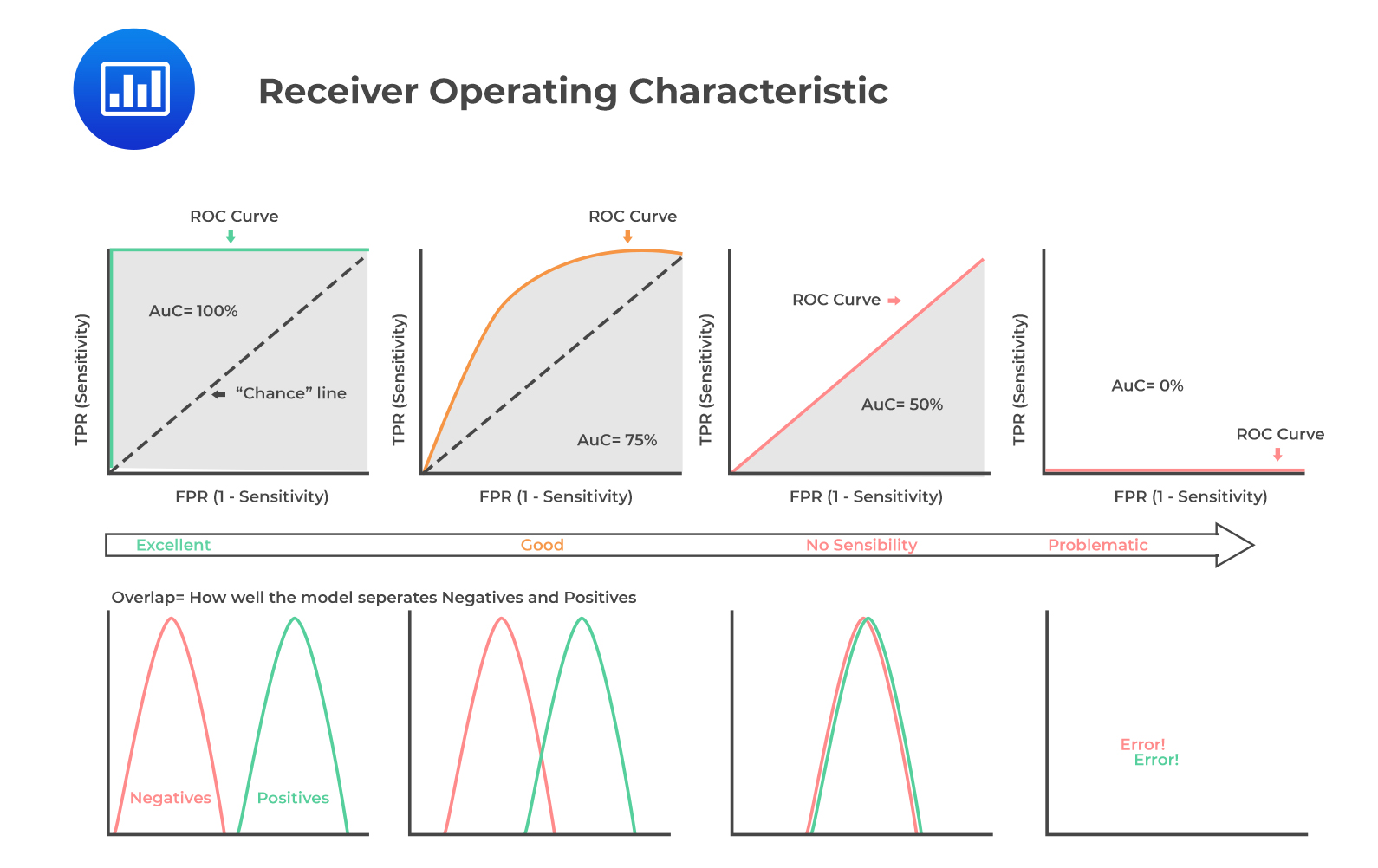The cleansed and preprocessed data set is split into three separate sets: training set, cross-validation (CV) set, and test set in the ratio 60:20:20, respectively.

The final document term matrix (DTM) is built using the sentences (rows), which are the instances, and resulting tokens (columns), which are the feature variables, from the BOW of the training dataset. The columns of DTMs for the splits are the same, equal to the number of unique tokens (i.e., features) from the final training corpus BOW.

A summary of the three data splits is shown in the following table:

$$\small{\begin{array}{|c|c|c|}\hline\textbf{Corpus} & \textbf{Split} (\%) & \textbf{Use} \\ \hline\text{Master} & 100\% & \text{Data exploration} \\ \hline\text{Training} & 60\% & \text{ML Model training} \\ \hline\text{Cross-validation} & 20\% & {\text{Turning and validating}\\ \text{the trained model}} \\ \hline\text{Test} & 20\% & {\text{Testing the trained,}\\ \text{tuned, and validated model}}\\ \hline\end{array}}$$

Method Selection

Sentiment analysis involves the use of textual data, which is more extensive with many possible variables and a known output, i.e., positive, neutral, or negative sentiment classes. A supervised ML algorithm, therefore, applies to sentiment analysis. ML algorithms such as SVM, decision trees, and logistic regression can also be examined in this case. For simplicity, we will assume that logistic regression is used to train the model.

In this case, we assume that texts are the sentences, and the classifications are either positive or negative sentiment classes (labeled 1 and 0, respectively). The tokens are feature variables, and the sentiment class is the target variable.

Logistic regression utilizes the method of maximum likelihood estimation. As a result, the output of the logistic model is a probability value ranging from 0 to 1. A mathematical function uses the logistic regression coefficient (β) to calculate the probability (p) of sentences having positive sentiment (y = 1). For example, if the p-value for a sentence is 0.90, there is a 90% probability that the sentence has a positive sentiment. We aim to find an ideal threshold value of p, which is a cutoff point for p values, and it depends on the dataset and model training.

When the p values are above the ideal threshold p-value, the sentences have a high probability of having a positive sentiment (y = 1). The ideal threshold p-value is estimated heuristically using performance metrics and ROC curves.

Performance Evaluation and Tuning

This step involves predicting the sentiments of the sentences in the training and cross-validation (CV) DTMs using the trained ML model. ROC curves are plotted for model evaluation. Recall that for ROC curves, the x-axis is a false positive rate, \(\frac{FP}{TN+FP}\), and the y-axis is a true positive rate, \(\frac{TP}{TP+FN}\).

The following figure shows sample ROC Curves of model results for Training and cross-validation data:

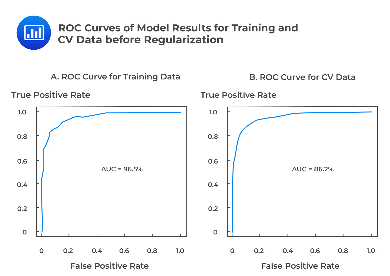The ROC curves are significantly different between the training and the CV datasets, i.e., the AUC is 96.5% on training data and 86.2% on CV data. This finding suggests that the model performs relatively poorly on the CV data when compared to training data, implying that the model is overfitted.

Regularization approaches such as least absolute shrinkage and selection operator (LASSO) are applied to the logistic regression model to mitigate the risk of overfitting. LASSO penalizes the coefficients of the model to prevent overfitting of the model. The penalized model only selects the tokens with statistically non-zero coefficients, and that contributes to the model fit.

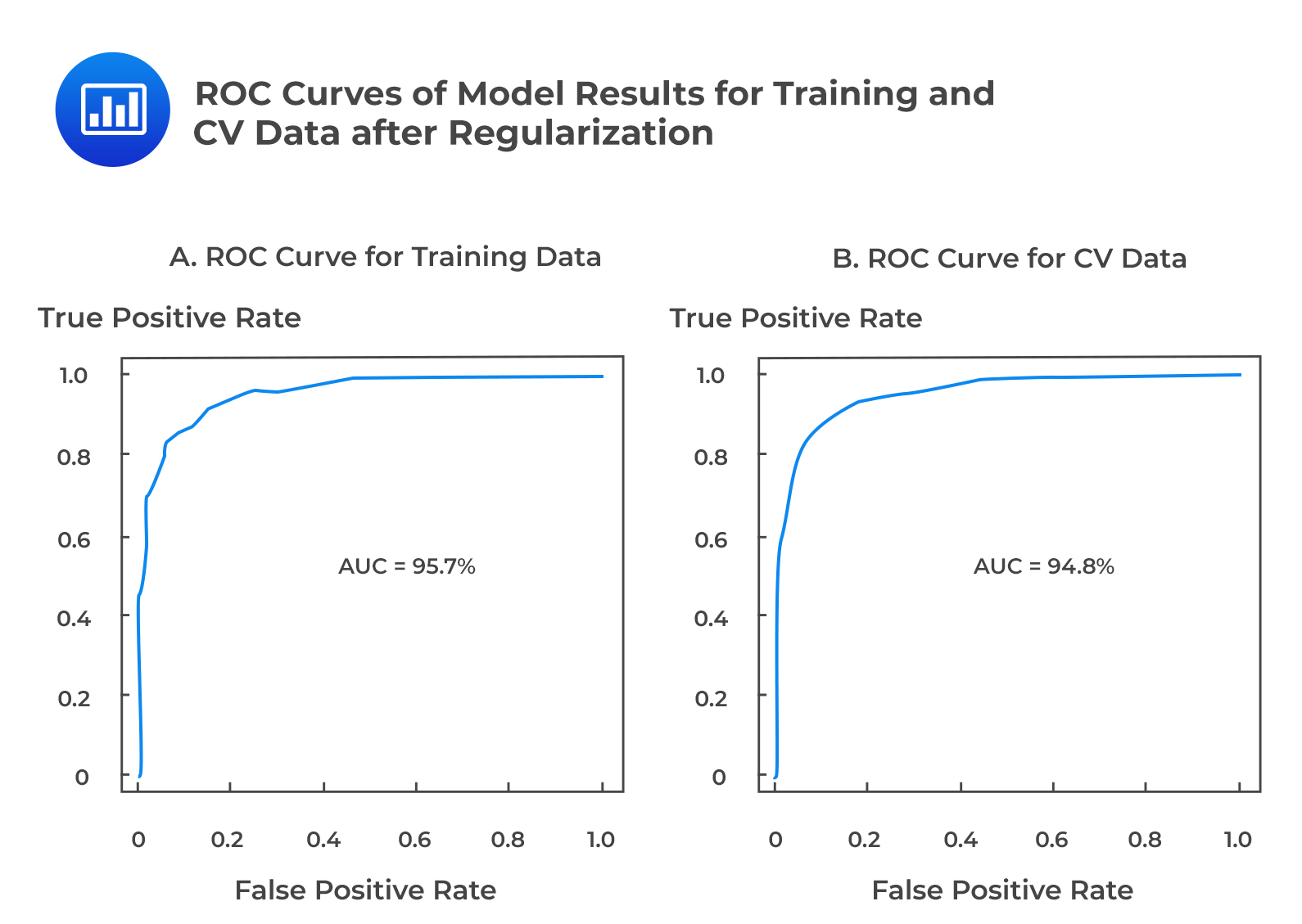The ROC curves are similar for model performance on both datasets, with an AUC of 95.7% on the training dataset and 94.8% on the CV dataset. This implies that the model performs almost identically on both training and CV data and thus indicates an excellent fitting model.

Error analysis can be used to evaluate the model further. It is performed by computing a confusion matrix using the ML model results from the CV dataset. The threshold p-value of 0.5 is the theoretically suggested threshold (cutoff). When p > 0.5, the prediction is assumed to be y = 1 (positive sentiment).

Confusion Matrix for CV Data with threshold p-value of 0.5

$$\small{\begin{array}{l|l|ll} {}& {}& \textbf{Actual Training Labels}&{}\\ \hline{}&{} & \text{Class “1.”} & \text{Class “0.”}\\ \hline\textbf{Predicted Results} & \text{Class “1”} & \text{TP} = 256 & \text{FP} = 27\\ {}& \text{Class “0”} & \text{FN} = 6 & \text{TN} = 103\\  \end{array}}$$

Performance Metrics

$$\begin{align*}\text{Precision (P)}&=\frac{\text{TP}}{\text{TP}+\text{FP}}\\&=\frac{256}{256+27}=0.9046\end{align*}$$

$$\begin{align*}\text{Recall (R)}&=\frac{\text{TP}}{\text{TP}+\text{FN}}\\&=\frac{256}{256+6}=0.9771\end{align*}$$

$$\begin{align*}\text{F1 score}&=\frac{(2\times\text{Precision}\times\text{Recall})}{\text{Precision}+\text{Recall}}\\&=\frac{2\times0.9046\times0.9771}{0.9046+0.9771}\\&=0.9394\end{align*}$$

$$\begin{align*}\text{Accuracy}&=\frac{TP+TN}{TP+FP+TN+FN}\\&=\frac{256+103}{256+27+6+103}\\&=0.9158\end{align*}$$

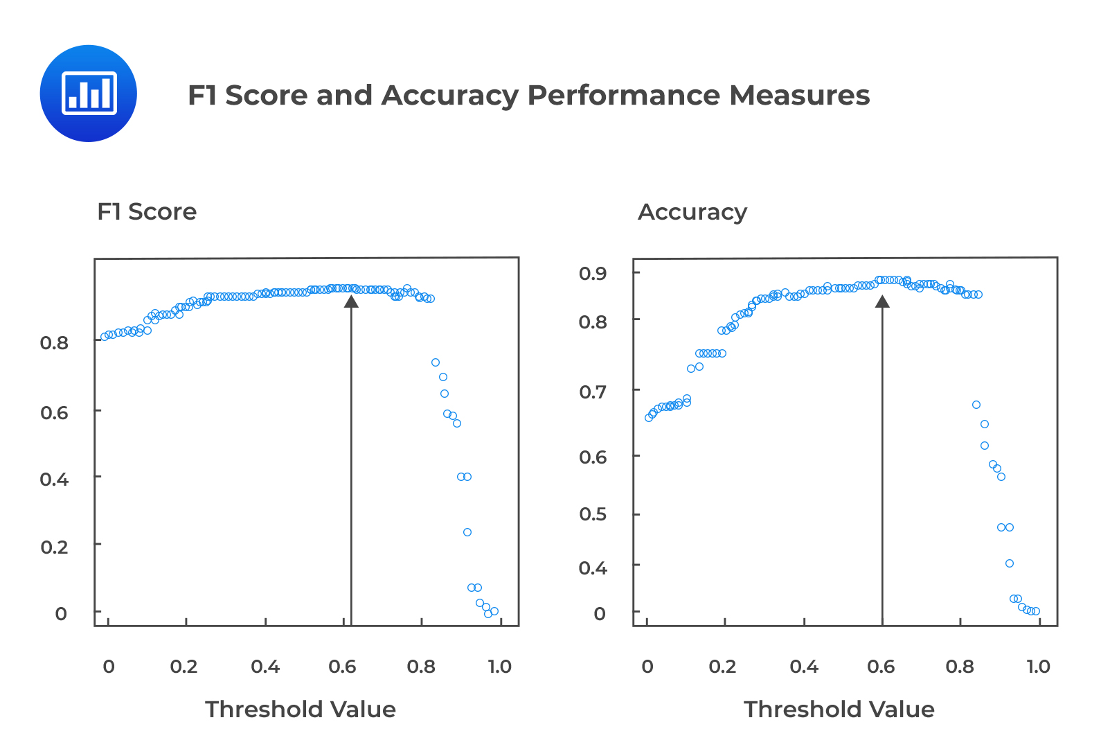
In this case, the model accuracy is 91.58%, with a theoretically suggested threshold p-value of 0.5. It is a standard practice to simulate many model results with different threshold values and to look for maximized accuracy and F1 statistics that minimize trade-offs between FP (Type I error) and FN (Type II error). What follows is to identify the threshold p-value that generates the highest accuracy and F1 score.

For example, the following figure shows the F1 score and accuracy performance measures for various threshold p values. The threshold p-value that results in the highest accuracy and F1 score can be identified as 0.6.

Confusion Matrix for CV Data with threshold p-value of 0.6

$$\small{\begin{array}{l|l|l|l} {}&{} &\textbf{Actual Training Labels}&{}\\ \hline{}& {}& \text{Class “1.”} & \text{Class “0.”}\\ \hline\textbf{Predicted Results} & \text{Class “1”} & \text{TP} = 256 & \text{FP} = 19 \\{} & \text{Class “0”} & \text{FN} = 6 & \text{TN} = 100\\  \end{array}}$$

Performance Metrics

$$\begin{align*}\text{Precision (P)}&=\frac{256}{256+19}\\&=0.9309\end{align*}$$

$$\begin{align*}\text{Recall (R)}&=\frac{256}{256+6}\\&=0.9771\end{align*}$$

$$\begin{align*}\text{F1 score}&=\frac{2\times0.9309\times0.9771}{0.9309+0.9771}\\&=0.9534\end{align*}$$

$$\begin{align*}\text{Accuracy}&=\frac{256+100}{256+19+6+100}\\&=0.9344\end{align*}$$

The model performance metrics improved in the final model relative to the earlier case when the threshold p-value was 0.5. With a threshold p-value of 0.6, the precision, accuracy, and F1 score have increased. The precision has increased by approximately 3% to 93%, while the accuracy and F1 score both increasing by approximately 1% to 93% and 95%, respectively.

Results and Interpretation

The final ML model, with the appropriate threshold p-value, has been validated and is now ready for application. It can be used to predict the sentiment of new sentences from the test data corpus as well as new sentences from almost identical financial text data sources. The model is now applied to the test data. Note that the test data has neither been used to train the model nor validate it.

The confusion matrix for the test data using a threshold p-value of 0.6 is as shown:

Confusion Matrix for Test Data with Threshold p-value of 0.6

$$\small{\begin{array}{l|l|l|l} {}&{} &\textbf{Actual Training Labels}&{}\\ \hline{}& {}& \text{Class “1.”} & \text{Class “0.”}\\ \hline\textbf{Predicted Results} & \text{Class “1”} & \text{TP} = 256 & \text{FP} = 24 \\{} & \text{Class “0”} & \text{FN} = 6 & \text{TN} = 107\\  \end{array}}$$

Performance Metrics

$$\begin{align*}\text{Precision (P)}&=\frac{256}{256+24}\\&=0.9413\end{align*}$$

$$\begin{align*}\text{Recall (R)}=\frac{256}{256+6}==0.9771\end{align*}$$

$$\begin{align*}\text{F1 score}&=\frac{2\times0.9413\times0.9771}{0.9413+0.9771}\\&=0.9313\end{align*}$$

$$\begin{align*}\text{Accuracy}&=\frac{256+107}{256+24+6+107}\\&=0.9237\end{align*}$$

From the confusion matrix for the test data, we get accuracy and F1 score of 92% and 93%, respectively, with precision and recall of 94% and 98%, respectively. Therefore, it is clear that the model performs similarly on the training, CV, and test datasets. Additionally, this implies that the model is robust and is not overfitting. It also suggests that the model generalizes well out-of-sample and can thus be used to predict the sentiment classes for new sentences from similar financial text data sources.

The following figure recaps the entire section of classifying and predicting sentiments using textual data from financial data sources.

The derived sentiment classification can be used to visualize insights regarding a large text without reading the entire document.

Question

In the previous analysis using the cross-validation dataset, the threshold value of 0.60 was determined to be the p-value that maximizes model accuracy and F1 score; the confusion matrix for this model is shown in Table A below:

Table A: Confusion Matrix for CV Data with Threshold p-value of 0.6

$$\small{\begin{array}{l|l|l|l} {}&{} &\textbf{Actual Training Labels}&{}\\ \hline{}& {}& \text{Class “1.”} & \text{Class “0.”}\\ \hline\textbf{Predicted Results} & \text{Class “1”} & \text{TP} = 256 & \text{FP} = 19 \\{} & \text{Class “0”} & \text{FN} = 6 & \text{TN} = 100\\  \end{array}}$$

You are given the following confusion matrix of the same model with threshold p values of 0.4, as shown in Table B below:

Table B: Confusion Matrix for CV Data with Threshold p-value of 0.4

$$\small{\begin{array}{l|l|l|l} {}&{} &\textbf{Actual Training Labels}&{}\\ \hline{}& {}& \text{Class “1.”} & \text{Class “0.”}\\ \hline\textbf{Predicted Results} & \text{Class “1”} & \text{TP} = 256 & \text{FP} = 30 \\{} & \text{Class “0”} & \text{FN} = 6 & \text{TN} = 106\\  \end{array}}$$

When the performance metrics of Table B (using a threshold p-value of 0.4) are compared with those of Table A (using a threshold p-value of 0.60), Table B is more likely to have a:

     A. Lower accuracy and a lower F1 score relative to Table A.

     B. Higher accuracy and a higher F1 score relative to Table A.

     C. Lower accuracy and the same F1 score relative to Table A.

Solution

The correct answer is A.

Performance metrics for confusion matrix A with threshold p-value of 0.6:

$$\begin{align*}\text{Precision (P)}&=\frac{256}{256+19}\\&=0.9309\end{align*}$$

$$\begin{align*}\text{Recall (R)}&=\frac{256}{256+6}\\&=0.9771\end{align*}$$

$$\begin{align*}\text{F1 Score}&=\frac{2\times0.9309\times0.9771}{0.9309+0.9771}\\&=0.9534\end{align*}$$

$$\begin{align*}\text{Accuracy}&=\frac{256+100}{256+19+6+100}\\&=0.9344\end{align*}$$

Performance metrics for confusion matrix B with a threshold p-value of 0.4:

$$\begin{align*}\text{Precision (P)}&=\frac{256}{256+30}\\&=0.8951\end{align*}$$

$$\begin{align*}\text{Recall (R)}&=\frac{256}{256+6}\\&=0.9771\end{align*}$$

$$\begin{align*}\text{F1 Score}&=\frac{2\times0.8951\times0.9771}{0.8951+0.9771}\\&=0.9343\end{align*}$$

$$\begin{align*}\text{Accuracy}&=\frac{256+106}{256+30+6+106}\\&=0.9095\end{align*}$$

It is clear that Table B has the same number of TPs (256) and TNs (106) as Table A. It follows that Table B also has lower accuracy (0.9095) and a lower F1 score (0.9343) relative to Table A. It is apparent that the ML model using the threshold p-value of 0.6 is the better model in this sentiment classification context with a threshold p-value of 0.4.

Reading 7: Big Data Projects

LOS 7 (g) Evaluate the fit of a machine learning algorithm