


A Review of Multiple Linear Regression ...
Multiple linear regression describes the variation of the dependent variable by using two... Read More

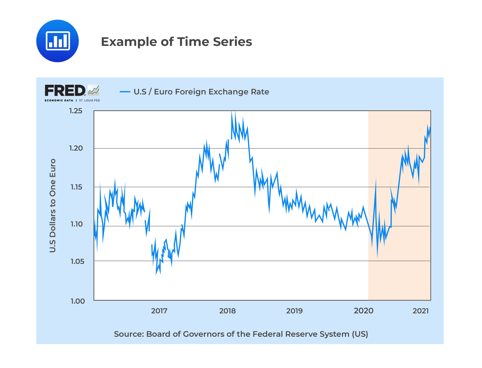
A time series shows data on a variable’s outcome in different periods—for example, a time series showing EURUSD exchange rates between a given time interval.
 Time series models explain the past and predict the future of a time series using a trend, which is a long-term pattern in a specific direction.
In a linear trend, the dependent variable changes at a constant amount with time. Consider a time series with a linear trend. The value of the time series at time \(t\) can be expressed as:
$$\text{y}_{\text{t}}=\text{b}_{0}+\text{b}_{1}\text{t}+\epsilon_{\text{t}}$$
Where:
\(\text{y}_{\text{t}}\) = Value of the time series at time \(t\).
\(\text{b}_{0}\) = Intercept term.
\(\text{b}_{1}\) = Trend coefficient.
\(\text{t}\) = Time, the independent variable. \(t=1, 2, …, \text{T}\).
\(\epsilon_{\text{t}}\) = Random error term.
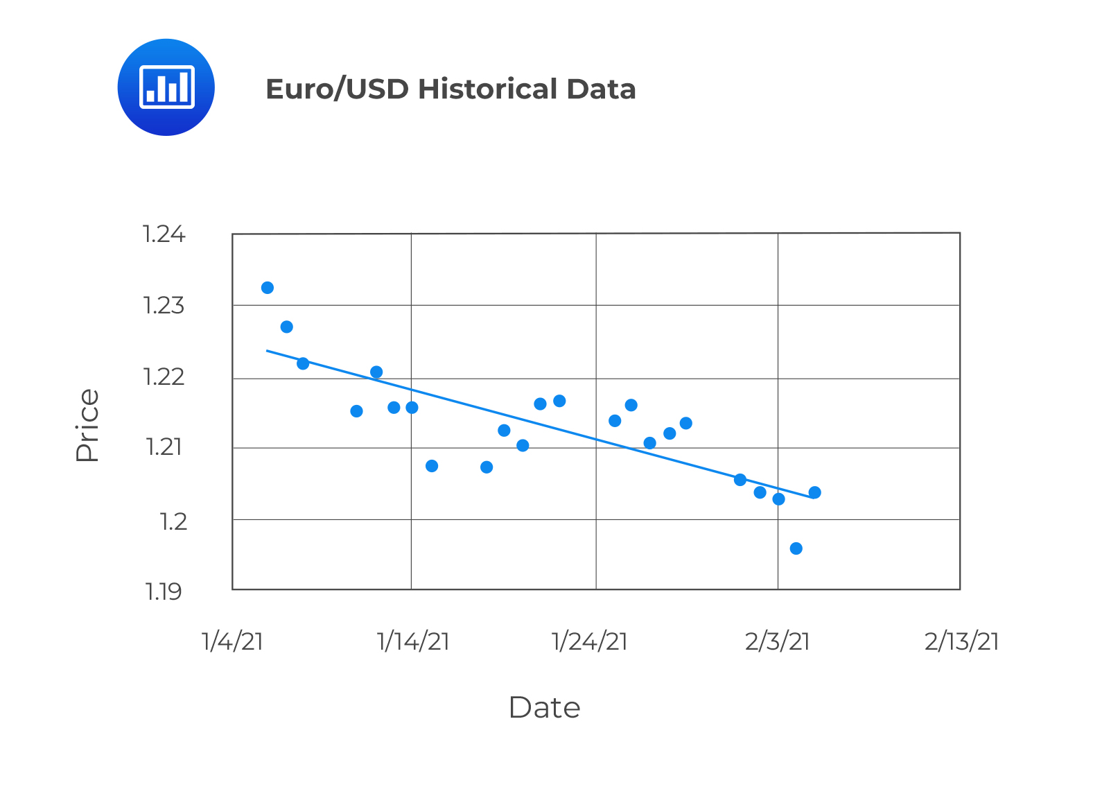
The following shows a linear trend of the EURUSD between 05 January 2021 to 06 February 2021.
 Predicted Value of a Linear Trend
The predicted value of a time series with a linear trend in period five is expressed as:
$$\widehat{y_{5}}=\widehat{b_{0}}+\widehat{b_{1}}(5)$$
The predicted value of a time series for period \(T+1\) is given by:
$$\widehat{\text{y}}_{T+1}=\widehat{b}_{0}+\widehat{b_{1}}(T+1)$$
Given that \(b_{0}=2\) and \(b_{1}=1.6\), the predicted value of y after four periods is closest to:
$$y_{t}=b_{0}+b_{1}t+\epsilon_{t}$$
$$y_{4}=2+1.6\times4=8.4$$
A log-linear trend analysis relies on an independent variable that changes exponentially over time or grows at a constant rate. It often works better with financial time series.
A time series with exponential growth can be modeled as:
$$y_{t}=e^{b_{0}+b_{1}(t)}$$
Where:
\(y_{t}\) = The value of the dependent variable at time \(t\).
\(b_{0}\) = Intercept term.
\(b_{1}\) = Constant growth rate.
\(t\) = time = \(1,2,3,…,T\).
Taking the natural log on both sides of the above equation generates a log-linear model expressed as:
$$\text{lny}_{\text{t}}=\text{ln ln}(e^{b_{0}+b_{1}t})$$
$$\text{ln ln}\ \text{y}_{\text{t}}=\ \text{b}_{0}+\text{b}_{1}\text{t}$$
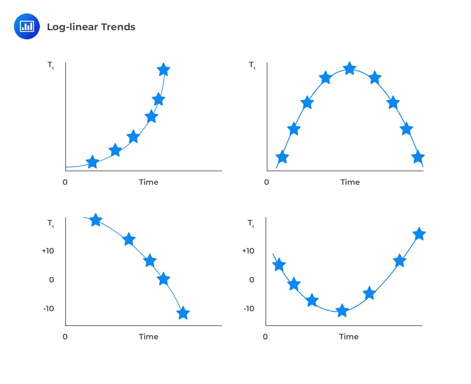
The following figure shows different forms of log-linear trends.
 Example: Predicted Value of a Log-Linear Trend
If \(b_{0}=3\) and \(b_{1}=1.5\), the predicted value of y after four periods is:
$$\text{ln y}_{t}=b_{0}+b_{1}t+\epsilon_{t}$$
$$\text{ln y}_{4}= 3+1.5\times4$$
$$\text{y}_{4}=e^{9}=8103.08$$
Question
Consider a log-linear trend model with an intercept term of 0.5 and a slope coefficient of 0.10. The predicted value of the trend after six periods is closest to:
A. 1.1.
B. 1.6.
C. 3.0.
Solution
The correct answer is C.
$$y_{t}=e^{b_{0}+b_{1}(t)}$$
$$y_{t}=e^{0.5+(0.10\times6)}=3.0$$
Reading 5: Time Series Analysis
LOS 5 (a) Calculate and evaluate the predicted trend value for a time series, modeled as either a linear trend or a log-linear trend, given the estimated trend coefficients.
Learn trend analysis, forecasting models, and time-series techniques with clear study tools.
Offered by AnalystPrep


Get Ahead on Your Study Prep This Cyber Monday! Save 35% on all CFA® and FRM® Unlimited Packages. Use code CYBERMONDAY at checkout. Offer ends Dec 1st.