Feature Extraction, Selection, and Engineering of Textual Data

Feature Extraction

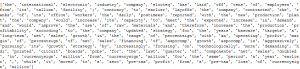
Feature extraction entails mapping the textual data to real-valued vectors. After the text has been normalized, the next step is to create a bag-of-words (BOW). It is a representation of analyzing text. It does not, however, represent the word sequences or positions.

The following figure represents a BOW of the textual data extracted from the Sentences_50Agree file for the first 233 words:

Feature Selection

Feature selection for text data entails keeping the useful tokens in the BOW that are informative and eliminating different classes of texts, i.e., those with positive sentiment and those with negative sentiment. The process of quantifying how important tokens are in a sentence and the corpus as a whole is known as frequency analysis. It assists in filtering unnecessary tokens (or features).

Term frequency (TF) is calculated and examined to pinpoint noisy terms, i.e., outlier terms. TF at the corpus level—also known as collection frequency (CF)—is the number of times a given word appears in the whole corpus divided by the total number of words in the corpus. Terms with low TF are mostly rare terms, for example, proper nouns or sparse terms, which rarely appear in the data and do not contribute to the differentiating sentiment. On the other hand, terms with high TF are mostly stop words, present in most sentences, so do not contribute to the differentiating sentiment. These terms are eliminated before forming the final document term matrix (DTM).

The next step involves constructing the DTM for ML training. Different TF measures are calculated to fill in the cells of the DTM as follows

1. SentenceNo: This is a unique identification number given to each sentence in the order they appear in the original dataset. For example, sentence number 11 is a sentence in row 11 from the data table.

2. TotalWordsInSentence: It is the count of the total number of words present in the sentence.

3. Word: This is a word token that is present in the corresponding sentence.

4. TotalWordCount: This is the total number of occurrences of the word in the entire corpus or collection.

$$\text{TF (Collection level)}=\frac{\text{TotalWordCount}}{\text{Total number of words in collection}}$$

5. WordCountInSentence: This refers to the number of times the token is present in the corresponding sentence. For example, in the sentence, “The profit before taxes decreased to EUR 31.6 million from EUR 50.0 million the year before.” The token “the” is present two times.

6. SentenceCountWithWord: This is the number of sentences in which the word is present.

7. Term Frequency (TF) at Sentence Level: This is the proportion of the number of times a word is present in a sentence to the total number of words in that sentence.

$$\text{TF at Sentence Level}=\frac{\text{WordCountInSentence}}{\text{TotalWordsInSentence}}$$

8. Document frequency (DF): This is calculated as the number of sentences that contain a given word divided by the total number of sentences. DF is essential since words frequently occurring across sentences provide no differentiating information in each sentence.

$$\text{DF}=\frac{\text{SentenceCountWithWord}}{\text{Total number of sentences}}$$

9. Inverse Document Frequency (IDF): This is a relative measure of how unique a term is across the entire corpus. A low IDF implies a high word frequency in the text

$$\text{IDF}=\text{log}\bigg(\frac{1}{\text{DF}}\bigg)$$

10. TF–IDF: TF at the sentence level is multiplied by the IDF of a word across the entire dataset to get a complete representation of the value of each word. High TF–IDF values indicate words that appear more frequently within a smaller number of documents. This signifies relatively more unique terms that are crucial. The converse is true. TF–IDF values can serve as word feature values for training an ML model

$$\text{TF}-\text{IDF}=\text{TF}\times\text{IDF}$$

Feature Engineering

Up to now, we have been dealing with single words or tokens, which, combined with the bag of words model, implied the assumption of independent words. One way of minimizing the effect of this simplification by adding some context to the words is to use n-grams. N-grams helps us to understand the sentiment of a sentence as a whole.

An n-gram refers to a set of n consecutive words that can be used as the building blocks of an ML model. Notice that we have been using the n-gram model for the particular case of n equals one, which is also called a unigram (for n=2, the n-gram model is a bigram, for n=3 trigram). When dealing with n-grams, unique tokens to denote the beginning and end of a sentence are sometimes used. Bigram tokens help keep negations intact in the text, which is crucial for sentiment prediction.

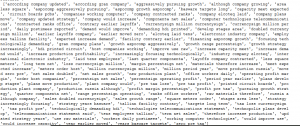
The corresponding word frequency measures for the DTM are then computed based on the new BOW formed from n-grams.

The following figure shows a sample of 3-gram tokens for the dataset sentences_50Agree for the first 233 words.

Example: Calculating and Interpreting Term Frequency Measures

Peter Smith is a data scientist and wants to use the textual data from sentences_50Agree file to develop sentiment indicators for forecasting future stock price movements. Smith has assembled a BOW from the corpus of text being examined and has pulled the following abbreviated term frequency measures tables. The text file has a total of 112,622 non-unique tokens that are in 4,820 sentences.

Term Frequency Measures Table 1

$$\small{\begin{array}{l|c|c|c|c|c} \text{Sentence No} & {\text{TotalWordsIn}\\ \text{Sentence}} & \text{Word} & {\text{TotalWord}\\ \text{Count}} & {\text{WordCountIn}\\ \text{Sentence}} & {\text{SentenceCount}\\ \text{WithWord}}\\ \hline <\text{int}>& <\text{int}> & <\text{chr}> & <\text{int}> & <\text{int}> & <\text{int}>\\ \hline7 & 43 & \text{a} & 1745 & 3 & 1373 \\ \hline4 & 34 & \text{the} & 6068 & 5 & 3678\\ \hline22 & 43 & \text{of} & 3213 & 3 & 2120\\ \hline22 & 43 & \text{the} & 6068 & 4 & 3678\\ \hline4792 & 28 & \text{a} & 1745 & 3 & 1373\\  \end{array}}$$

Term Frequency Measures Table 2

$$\small{\begin{array}{l|c|c|c|c|c} \text{SentenceNo} & {\text{TotalWordsIn}\\ \text{Sentence}} & \text{Word} & {\text{TotalWord}\\ \text{Count}} & {\text{WordCountIn}\\ \text{Sentence}} & {\text{SentenceCount}\\ \text{WithWord}}\\ \hline<\text{int}> & <\text{int}> & <\text{chr}> & <\text{int}> & <\text{int}> &<\text{int}>\\ \hline4 & 34 & \text{increase} & 103 & 3 & 100\\ \hline647 & 27 & \text{decrease} & 11 & 1 & 11\\ \hline792 & 12 & \text{great} & 6 & 1 & 6\\ \hline4508 & 47 & \text{drop} & 7 & 1 & 7\\ \hline33 & 36 & \text{rise} & 17 & 1 & 17\\  \end{array}}$$

1. Determine and interpret term frequency (TF) at the collection level and at the sentence level for the token “the” in sentence 4 in term frequency measures Table 1.
2. Determine and interpret term frequency (TF) at the collection level, and the sentence level for the token “decrease” in sentence 647 in term frequency measures Table 2.
3. Determine and interpret TF–IDF (term frequency-inverse document frequency) for the token “the” in sentence 4 in term frequency measures Table 1.

Solution to 1:

$$\begin{align*}\text{TF (Collection Level)}&=\frac{\text{Total Word Count}}{\text{Total number of words in collection}}\\&=\frac{6,068}{112,622}\\&=5.39\%\end{align*}$$

TF at the collection level is an indicator of the frequency that a token is used throughout the whole collection of texts (here, 112,622). It is vital for identifying outlier words: Tokens with the highest TF values are mostly stop words that do not contribute to differentiating the sentiment embedded in the text (such as “the”).

$$\begin{align*}\text{TF at Sentence Level}&=\frac{\text{Word Count In Sentence}}{\text{Total Words In Sentence}}\\&=\frac{5}{34}\\&=0.1471 \ or \ 14.71\%\end{align*}$$

TF at the sentence level is an indicator of the frequency that a token is used in a particular sentence. Therefore, it is useful for understanding the importance of the specific token in a given sentence.

Solution to 2:

For the token “decrease,” the term frequency (TF) at the collection level is given by:

$$=\frac{11}{112,622}=0.0098\%$$

This token has a meager TF value. Recall that tokens with the lowest TF values are mostly proper nouns or sparse terms that are also not important to the meaning of the text.

$$\begin{align*}\text{TF at Sentence Level for the token “decrease”}&=\frac{1}{27}\\&=0.037 \ or \ 3.70\%\end{align*}$$

TF at the sentence level is an indicator of the frequency that a word is used in a particular sentence. Therefore, it is useful for understanding the importance of the specific token in a given sentence.

Solution to 3:

To calculate TF–IDF, document frequency (DF) and inverse document frequency (IDF) also need to be calculated.

$$\text{DF}=\frac{\text{Sentence Count with Word}}{\text{Total number of sentences}}$$

For token “the” in sentence 4,

$$\begin{align*}\text{DF}&=\frac{3,678}{4,820}\\&=0.7631or76.31\%\end{align*}$$

Document frequency is important since tokens frequently occurring across sentences (such as “the”) provide no differentiating information in each sentence.

IDF is a relative measure of how important a term is across the entire corpus:

$$\text{IDF}=\text{log}\bigg(\frac{1}{\text{DF}}\bigg)$$

For token “the” in sentence 4:

$$\begin{align*}\text{IDF}&=\text{log}\bigg(\frac{1}{0.7631}\bigg)\\&=0.2704\end{align*}$$

Using TF and IDF, TF–IDF can now be calculated as:

$$\text{TF}-\text{IDF}=\text{TF}\times\text{IDF}$$

For token “the” in sentence 4, \(TF-IDF=0.1471\times0.2704=0.0398 \ or \ 3.98%\)

As TF–IDF combines TF at the sentence level with IDF across the entire corpus, it provides a complete representation of the value of each word. A low TF–IDF value indicates tokens that appear in most of the sentences and are not discriminative (such as “the”). TF–IDF values are useful in extracting the key terms in a document for use as features for training an ML model.

Question

The TF–IDF (term frequency-inverse document frequency) for the token “decrease” in sentence 647 in term frequency measures Table 2 is most likely:

      A. 19.64%.

      B. 20.58%.

      C. 22.53%.

Solution

The correct answer is C.

To calculate TF–IDF, document frequency (DF), and inverse document frequency (IDF) also need to be calculated.

$$\text{DF}=\frac{\text{Sentence Count With Word}}{\text{Total number of sentences}}$$

For token “decrease” in sentence 647,

$$\begin{align*}\text{DF}&=\frac{11}{4,820}\\&=0.00228or0.228\%\end{align*}$$

Document frequency is important since tokens frequently occurring across sentences (such as “the”) provide no differentiating information in each sentence.

IDF is a relative measure of how important a term is across the entire corpus.

$$\text{IDF}=\text{log}\bigg(\frac{1}{\text{DF}}\bigg)$$

For token “decrease” in sentence 647:

$$\begin{align*}\text{IDF}&=\text{log}\bigg(\frac{1}{0.00228}\bigg)\\&=6.083\end{align*}$$

Using TF and IDF, TF-IDF can now be calculated as:

$$\text{TF}-\text{IDF}=\text{TF}\times\text{IDF}$$

For token “the” in sentence 647, \(\text{TF}-\text{IDF}=0.037\times6.083=0.2253, or 22.53\%\)

As TF–IDF combines TF at the sentence level with IDF across the entire corpus, it provides a complete representation of the value of each word. A high TF–IDF value indicates the word appears many times within a small number of documents, signifying an important yet unique term within a sentence (such as “decrease”).

Reading 7: Big Data Projects

LOS 7 (f) Describe methods for extracting, selecting and engineering features from textual data