Mean-Variance Portfolio Theory

After completing this reading, you should be able to:

1. Explain the mathematics and summary statistics of portfolios.
   • Calculate the risk and return of an asset, given appropriate inputs.
   • Calculate the risk and expected return of a portfolio of many risky assets, given the expected return, volatility and correlation of returns of the individual assets. 
2. Perform mean-variance analysis.
   • Understand the mean-standard deviation diagram and the resulting efficient market frontier.
   • Calculate the optimal portfolio and determine the location of the capital market line.
   • Understand how portfolio risk can be reduced through diversification across multiple securities or across multiple asset classes.

The Challenge Facing Rational Investors

In a given market, an investor is presented with different assets/securities with different levels of return based on the underlying risk.

A practical consideration rational investors face is how best to select the asset or combination of assets or security investments that present an optimal balance between risk and return on investment and maximizes their expected utility.

The Mean-Variance Portfolio Theory (MPT)

Harry Markowitz conceptualized the Mean-Variance Portfolio Theory, also known as The Modern Portfolio Theory, in 1952. Through the concepts presented in theory, investors can draw practical guides into constructing investment portfolios that maximize their expected return based on a given level of risk.

Definitions

We define some of the basic terms which we will be using in the context of the Modern Portfolio Theory:

Risk: In the context of MPT, risk can be defined as the variance or deviation of the investment return from the level expected.

Return: This is the reward an investor earns from investing/committing their capital to a given asset/security.

Portfolio: A portfolio is a collection of assets such as stocks, property, bonds, currencies, etc.

Opportunity set: This is the set of available portfolios that an investor can choose based on their combinations of risk and return.

Diversification: Diversification is the process of mixing different assets within a portfolio to ensure that unsystematic risk is smoothed out. In this case, the negative performance of a given asset/security within the portfolio is balanced out by the positive performance of other assets within the portfolio.

The Theory

The principle theory behind the diversification concept is that investors should hold portfolios and focus on the relationship between the individual securities within the portfolio.

The assumption made by the theory is that the investment decisions are solely made with regard to the mean and variance of the investment return.

Thus, when applying the MPT framework to the selection of investment portfolios, the investor should consider the properties (i.e., the risk and return) of the available investment portfolios, the opportunity set, and out of these, choose the most efficient portfolios, also called the efficient frontier from the set.

Generally, the MPT tries to explain a method of constructing a portfolio that generates a maximum return for a given level of risk or a minimum risk for a stated return using the investor’s utility, which is assumed to be known. The investor tries to find the optimal balance between the return and the risk involved in the investment.

Although MPT has some limitations, it continues to be a cornerstone for portfolio managers by applying statistical techniques to portray to investors the benefits of diversification.

Assumptions of Modern Portfolio (Mean-Variance Portfolio) Theory

The Modern Portfolio theory relies on some strong assumptions, as listed below

• Markets are efficient, and investors have access to all the available information regarding the expected return, variances, and covariances of securities or assets.
• Investors are risk-averse, i.e., they will tend to avoid unnecessary risks. For example, investors choose to invest in bank deposits that pay lower returns but guaranteed returns rather than investing in stocks that may promise high returns but carry a high risk of losses.
• Investors are non-satiated, i.e., given two securities with the same standard deviation, an investor would choose the highest expected return.
• There is a fixed single-time horizon.
• There are no taxes or transaction costs.
• Assets can be held at any amount.
• A risk-free rate of return exists in the market, and unlimited capital can be borrowed or invested at this rate.
• Investors make their decisions solely based on expected returns and variance.

Mathematics and Statistics of Portfolios

Since a portfolio is a collection of assets or securities, it is clear that for us to find the expected return on a portfolio, we must know the mean and the variance and covariance of each security included in the collection. This leads us to the mathematics and statistics of portfolios.

In choosing the set of portfolios, where we are determined to find efficient portfolios, it is assumed that the investors make their decisions based on the expected return and variance of the returns over a single time unit. Therefore, we can stick to these two measures. A point to note here, however, is that the variance of any portfolio is equivalent to its risk.

Calculating the Return and Risk of an Asset

Return of an Asset

Let \(R_i\)represent the return generated by asset \(A\) in state \(i\) and \(p_i\) represent the likelihood of state \(i\) happening.

The expected return on the asset, \(E(A)\) can be computed as below:

$$E(A)=\sum_{\forall_i}{p_iR_i}$$

Example: Calculating the expected return of an asset

Over the next 1 year, the returns on stock J are expected to be 8% with a probability of 0.7 and 10% with a probability of 0.3.

Calculate the Expected return on Stock J

Solution

The expected return can be computed as:

$$ E (J)=\sum_{\forall_i}{p_iR_i} = 0.08\times0.7+0.1\times0.3=0.086=8.6\%$$

Risk of an Asset

The risk of an asset is measured by the standard deviation. Let \(R_i\) represent the return generated by asset \(A\) in state \(i\) and let \(p_i\) represent the likelihood of state \(i\) happening.The standard deviation of the asset,  can be computed as below:

• Compute the expected return on the asset as described previously.
• Multiply \(p_i\) by the square of each respective \(R_i\) to obtain \(E(A^2)\).
• Subtract \((E(A))^2\) from \(E(A^2)\) to obtain the variance of returns.
• Obtain the square root of the variance

Hence:

$$ \sigma_A=\sqrt{E(A^2)-\left(E\left(A\right)\right)^2}$$

Example: Calculating the Standard Deviation of an asset

Over the next 1 year, the returns on stock J is expected to be 8% with probability 0.7 and 10% with probability 0.3.

Calculate the Standard deviation of Stock J:

Solution

The standard deviation can be computed as:

$$\sigma_J=\sqrt{E(J^2)-\left(E(J)\right)^2}$$

Where

$$E(J)=\sum_{\forall_i}{p_iR_i=0.08\times0.7+0.1\times0.3=0.086}$$

$$E(J^2)=\sum_{\forall_i}{p_i\left(R_i\right)^2={0.08}^2\times0.7+{0.1}^2\times0.3=0.00743}$$

Thus,

$$\sigma_J=\sqrt{0.00743-\left({0.086}^2\right)}=0.009165$$

Expected Return and Risk of a Portfolio

Expected Return of a Portfolio

Suppose an investor has $1 to invest in any of the available securities in the market and that \(w_j\) represents the proportion of the available funds invested in asset \(j\) where \(j = 1,2,\ddots, N\).

If we denote the return of the portfolios by \(R_p\), then the return on the portfolio is given by:

$$ R_p=\sum _{ \forall j }^{ }{ w_j R_j } $$

Where:

\(R_p\) = The return on a portfolio;
\(w_j\) = The weight of funds to be invested; and
\(R_j\) = The return on asset \(j\).

Note that:

$$ \sum _{ \forall j }^{ }{ w_j }=1 $$

Now denote the expected return on a portfolio by \(E_p\), the expected return on a portfolio is given by:

$$ \begin{align*} E_p & =E(R_p )=E \left( \sum _{ \forall j }^{ }{ w_j R_j } \right) \\ & =\sum _{ \forall j }^{ }{ w_j E \left(R_j\right) } \\ & =\sum _{ \forall j }^{ }{ w_j E_j } \\ \end{align*} $$

So,

$$ E_p=\sum _{ \forall j }^{ }{ w_j E_j } $$

Where:

\(E_j\) = The expected return on each asset \(j\).

It is then clear that the expected return of a portfolio is the weighted mean of the individual securities’ expected returns.

Example: Calculating the expected return of a portfolio

An investor has constructed a portfolio of two assets, Asset A and asset B. The expected return of asset A is 8%, and the Expected return of asset B is 10%.

Calculate the Expected return on the portfolio if 65% of the funds is invested in asset A and the rest in asset B:

Solution

$$E_{P\ }=\sum_{\forall_i}{w_iR_i}=0.08\times0.65+0.1\times0.35=0.087=8.7\%$$

Risk of a Portfolio

The variance of the return on a portfolio is given by:

$$ \sigma^2=Var(R_p )=\sum _{ j }^{ }{ \sum _{ k }^{ }{ { w }_{ j }{ w }_{ k }{ C }_{ jk } } } $$

Where:

\(C_{jk}\) = The covariance between assets \(j\) and \(k\).

For illustration, consider two securities or assets A and B with expected returns \(E_A\) and \(E_B\) and variances \(\sigma_{A}^{2}\) and \(\sigma_{B}^{2}\). Let the weights be \(w_A\) and \(w_B\) respectively. Then, applying the formulas above:

$$ E_p=w_A E_A+w_A E_B $$

And

$$ \text {Portfolio variance} ,\sigma_p^2= w_A^2 \sigma_A^2+ w_B^2 \sigma_B^2+2w_A w_B \sigma_A \sigma_B \rho_{AB} $$

Where:

\(w\) = The weight of the asset within the portfolio;
\(\sigma\) = The standard deviation (which is a measure of volatility);
\(\rho\) = The correlation coefficient.

Note that:$$\sigma_A \sigma_B \rho_{AB} = \text {Cov}(A,B)$$

The portfolio standard deviation or variance, which is simply the square of the standard deviation, comprises of two key parts: the variance of the underlying assets plus the covariance of each underlying asset pair as shown above.

Also, given the portfolio variance equation above, we can deduce that the lower the covariance between the assets/securities returns, the lower the overall variance of the portfolios. This implies that investing in assets/securities whose returns are uncorrelated lowers the variance of a portfolio, which is the goal of diversification.

Example 1: Standard Deviation of a Portfolio

Consider a two-asset portfolio where asset A has an allocation of 80% and a standard deviation of 16%, and asset B has an allocation of 20% and a standard deviation of 25%. The correlation coefficient between assets A and B is 0.6.

Calculate the portfolio standard deviation.

Solution

We make use of  our portfolio variance equation introduced in the previous section:

$$\text{Portfolio variance},\sigma_p^2=w_A^2 \sigma_A^2+ w_B^2 \sigma_B^2+2w_A w_B\sigma_A \sigma_B \rho_{AB}$$

Where:

\(w_A  = 0.8, w_B = 0.2\)

\(\sigma_A=0.16, \sigma_B=0.25\)

\(\rho_{AB} = 0.6\)

Replacing the formula for values we get our portfolio variance as:

\begin{align*} \text{Portfolio variance} & = (0.8)^2 \times (0.16)^2+ (0.2)^2 \times (0.25)^2+ 2(0.8)(0.2)(0.16)(0.25)(0.6) \\ & =0.0266 \end{align*}

We know that the standard deviation is equal to the square root of the variance. Thus,

$$\text{Portfolio standard deviation} = \sqrt {0.0266} =0.163= 16.3\%  $$

Example 2: Standard Deviation of the Returns

The probability distribution of the return earned by a newly established hedge fund is as follows:

$$ \begin{array}{c|c} \textbf{Probability} & \textbf{Return(%)} \\ \hline \text{20%} & \text{8} \\ \text{40%} & \text{15} \\ \text{30%} & \text{20} \\ \text{10%} & \text{30} \\ \end{array} $$

Calculate the standard deviation of the returns of the hedge fund.

Solution

First.

We know that,

$$ Var(R)  = E(R^2) – \mu^2= E(R^2) – [E(R)]^2 $$

When presented with a range of returns together with their respective probabilities, the expected return can be computed using the below formula where \(r_i\) and \(p_i\) represent the individual returns and their probabilities, respectively.

$$E\left(R\right)=\sum_{\forall}{r_i p_i }$$

Applying the above formula we have,

$$E(R)  = 0.2×8 + 0.4×15 + 0.3×20 + 0.1×30 = 16.6$$

Using the same convention from above, we recall that,

$$E\left(R^2 \right)=\sum_{\forall}{r_i^2  p_i }$$

Thus,

$$\begin{align*}E(R^2) & = 0.2×8^2 + 0.4×15^2 + 0.3×20^2 + 0.1×30^2 = 312.8 \\ Var(R) & = 312.8 – 16.6^2 = 37.24\%\% \\ \Rightarrow \text {Standard deviation of return} = 37.24^{0.5} = 6.102\% \\ \end{align*} $$

Example 3: Portfolio Standard Deviation

The table below gives information about two assets.

$$ \begin{array}{c|c|c} \text{} & \textbf{Asset 1} & \textbf{Asset 2} \\ \hline \textbf{Weights} & \text{80%} & \text{20%} \\ \textbf{Expected Return} & \text{9.98%} & \text{15.80%} \\ \textbf{Standard Deviation} & \text{17.00%} & \text{30.00%} \\ \textbf{Covariance} & \text{0.005} & \text{} \\ \end{array} $$

Calculate the expected return and the standard deviation of a portfolio made up of the two assets

Solution

$$ \begin{align*} \text{Portfolio return} & = \text {weighted return of assets} \\ E(R_p) & = (0.8 × 9.98\%) + (0.2 × 15.8\%) = 11.14\% \\ \end{align*} $$ $$ \begin{align*} \text{Portfolio variance} (\sigma_p^2) & = w_1^2 \sigma_1^2 + w_2^2 \sigma_2^2 + 2w_1 w_2 \rho_{12} \sigma_1 \sigma_2 \\ & = 0.8^2 × 0.17^2 + 0.2^2 × 0.3^2 + 2 × 0.8 × 0.2 × 0.005 \\ & = 0.023696 \\ \end{align*} $$ $$ \text{Portfolio risk} =\text {Portfolio standard deviation} = \sqrt {0.023696} = 0.1539 = 15.39\% $$

Note: The portfolio risk is less than the risk of each respective asset highlighting the benefit of diversification.

Mean-Variance Analysis

We have so far explored how we can calculate the expected return and variance of a portfolio given a collection of assets. Next is to understand how an investor can select an efficient portfolio out of a given opportunity set.

In theory, a portfolio is made up of all investable assets. However, this is not practical, and thus, we must find a way of filtering the investable universe.

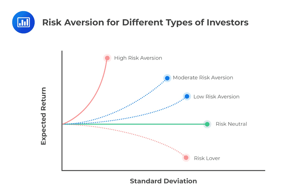
The assumption here is that we are considering a risk-averse investor, i.e., an investor who seeks to find the combination of portfolio assets that minimizes risk for a given level of return, or, maximize return for a given level of risk.

Mean Standard Deviation Diagram and the Efficient Market Frontier

Let us consider an investor presented with securities A and B below and has to make an investment decision based on their return and risk. How should the investor choose a portfolio of these two securities?

$$ \begin{array}{c|c|c}  \textbf{Security} & \textbf{Return} &\textbf{Standard Deviation}\\ \hline \textbf{A} & \text{10%} & \text{20%} \\ \hline \textbf{B} & \text{16%} & \text{35%} \\ \end{array} $$

Assume that 40% of the total funds total funds is invested in security A and 60% invested in security B. The expected return of the portfolio of these two assets can be computed as:

$$E(R_P)=(0.4\times 10\%)+(0.6\times 16\%)=13.60\%$$

Assume that the two securities are uncorrelated, i.e., with a correlation coefficient of zero, we can compute the variance of the portfolio as:

$$Var(R_P )= 0.4^2 (0.2)^2 +0.6^2 (0.35)^2=0.0505$$

Note: The covariance of uncorrelated securities is equal to zero.

Thus, the resulting standard deviation of the portfolio is\(\sqrt{0.0505}=22.47\%\)

We observe that investing in the two securities reduces the volatility of the returns of security B. However, the above allocation seems somewhat inefficient as it may be possible to construct a portfolio of the two assets in a manner that leads to the attainment of better terms for the investor in terms of risk and return. An investor obtains the best optimal return for minimal risk.

Specifically, we are trying to construct an efficient portfolio. For instance, we can consider investing 60% of the total funds in security A and 40% in security B, which will result in an overall portfolio standard deviation of 18.44% and an expected return of 12.40%. Thus, we can derive an investment opportunity set of different portfolio compositions that match the investor’s expected utility by varying the allocation to the underlying assets. Here the different blue lines represent different investor’s utility functions:

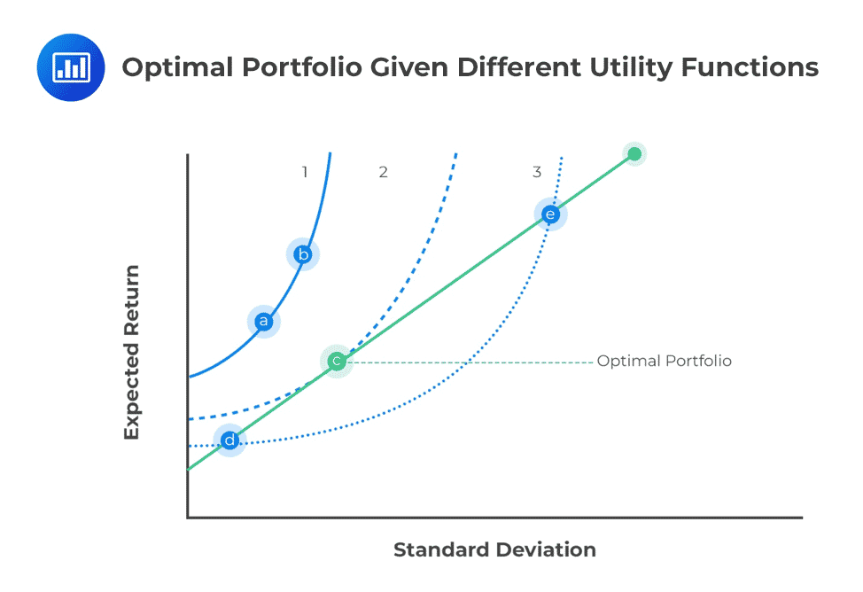To find the optimal portfolio, we make use of the investor’s indifference curve. This is made up of the various combinations of risky assets that lead to specific portfolio risk-return characteristics, graphically plotted with portfolio expected return on the y-axis and portfolio standard deviation on the x-axis.

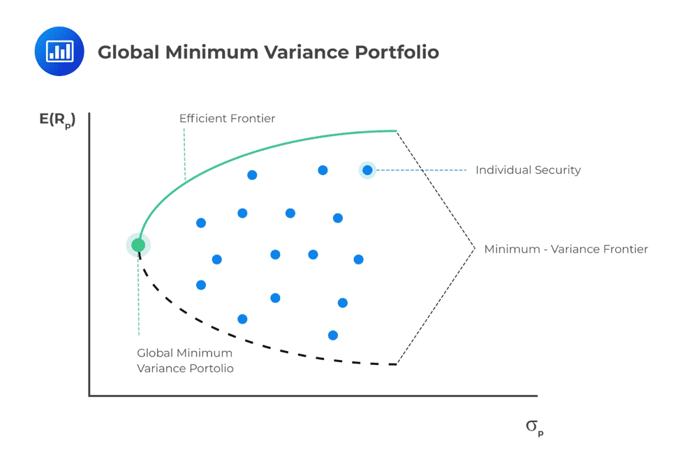
For each level of return, the portfolio with the minimum risk will be selected by a risk-averse investor. This minimization of risk for each level of return creates a minimum-variance frontier – a collection of all the minimum variance (minimum standard deviation) portfolios. There is a minimum-variance portfolio that produces the highest returns per unit of risk at a point along this minimum-variance frontier curve.

Global Minimum-variance Portfolio

Along the minimum-variance frontier, the left-most point is a portfolio with minimum variance compared to all possible collections of risky assets. This is known as the global minimum-variance portfolio. An investor cannot hold a portfolio of risky (note: risk-free assets are excluded at this point) assets with a lower risk than the global minimum-variance portfolio.

Efficient Frontier

The portion of the minimum-variance curve that lies above and to the right of the global minimum variance portfolio is known as the Markowitz efficient frontier. Along the efficient frontier line, rational risk-averse investors can select different portfolio sets that match their expected utility. All other combinations out of the efficient frontier line are inefficient.

Interestingly, we can monitor the slope of the efficient frontier, i.e., the change in units of return per unit of risk. As we move to higher levels of risk, the resulting increase in return begins to diminish. The slope begins to flatten. This means we cannot achieve ever-increasing returns as we take on more risk, quite the opposite of our expectations.

In the return-standard deviation curve, a series of indifference curves may be plotted so that the portfolios lying on the same curve have the same value of expected utility. By combining the investor’s indifference curves, an optimal portfolio can be constructed.

Calculating the Optimal Portfolio

Consider a portfolio made up of assets A and B. Let \(\sigma_A\) and \(\sigma_B\) represent the standard deviation of the assets, respectively. Also, let \(w_A\) and \(w_B\) represent the proportion of funds invested in each asset. We describe below how we can make the portfolio of the two assets optimal.

An optimal portfolio minimizes risk for a given level of return. The optimal portfolio is created by investing the right proportion of funds in the respective assets making up the portfolio. To calculate the optimal portfolio, we, therefore, need to compute the appropriate asset allocations that ensure minimum risk.

To determine the asset allocation that minimizes portfolio risk, we differentiate the portfolio variance equation with respect to the weight of that specific asset. We then equate the first derivative to zero and solve for the minimum point. For example, if we are interested in finding the value \(w_A\) that minimizes portfolio risk, we will differentiate the portfolio variance below with respect to \(w_A\):

$$\sigma_P^2=w_A^2\sigma_A^2+(1-w_A)^2\sigma_B^2+2w_A(1-w_A){\rm Cov}_{AB}$$

Differentiating, equating to zero, and solving for \(w_A\) we get:

$$W_A=\frac{\sigma_B^2-Cov(A,B)}{{(\sigma}_A^2+\sigma_B^2-2Cov{AB})}$$

This gives the asset allocation that creates an optimal portfolio of the two assets

The Capital Market Line

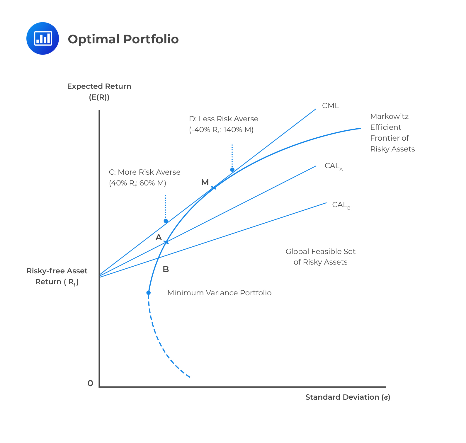
The capital market line is the tangent of the efficient frontier. The Modern Portfolio Theory forms the basis for the Capital Asset Pricing Model (to be covered later in the course) upon which the capital market line draws its form.

The Capital Market Line (CML) expresses the portfolio’s expected return as a linear function of the risk-free rate, the portfolio’s standard deviation, and the market portfolio’s return and standard deviation.

The market portfolio is the point on the efficient frontier where the line from the risk-free asset(where the risk is 0) is tangent to the efficient frontier. All the assets below the efficient frontier are inefficient portfolios since they provide the same level of return with a higher level of risk or a lower level of return with the same amount of risk. On the other hand, the points above the CML are not attainable.

All rational investors will hold the combination of the risk-free assets and M, the portfolio of risky assets, at the point where the capital market line touches the efficient frontier.

With this, we can determine the combination of an investor’s optimal portfolio without knowing their individual levels of risk aversion because the portfolio of risky assets for each investor will always be the market portfolio.

The risk-return characteristics as given by CML can be computed using a two-asset portfolio: A risk-free and a risky asset.

We explore the CML equation, which is given by:

$$ E(R_C )=R_f+ \left[\cfrac {E(R_m )-R_f}{\sigma_m} \right] \sigma_C $$

Where:

\(E(R_C )\) = The expected return on any portfolio;
\(R_f\) = The risk-free rate of return;
\(E(R_m )\) = The expected return on market portfolio;
\(\sigma_m\) = The standard deviation of the return; and
\(\sigma_C\) = The standard deviation on the return of the portfolio.

The equation above can be easily found from the graph below.

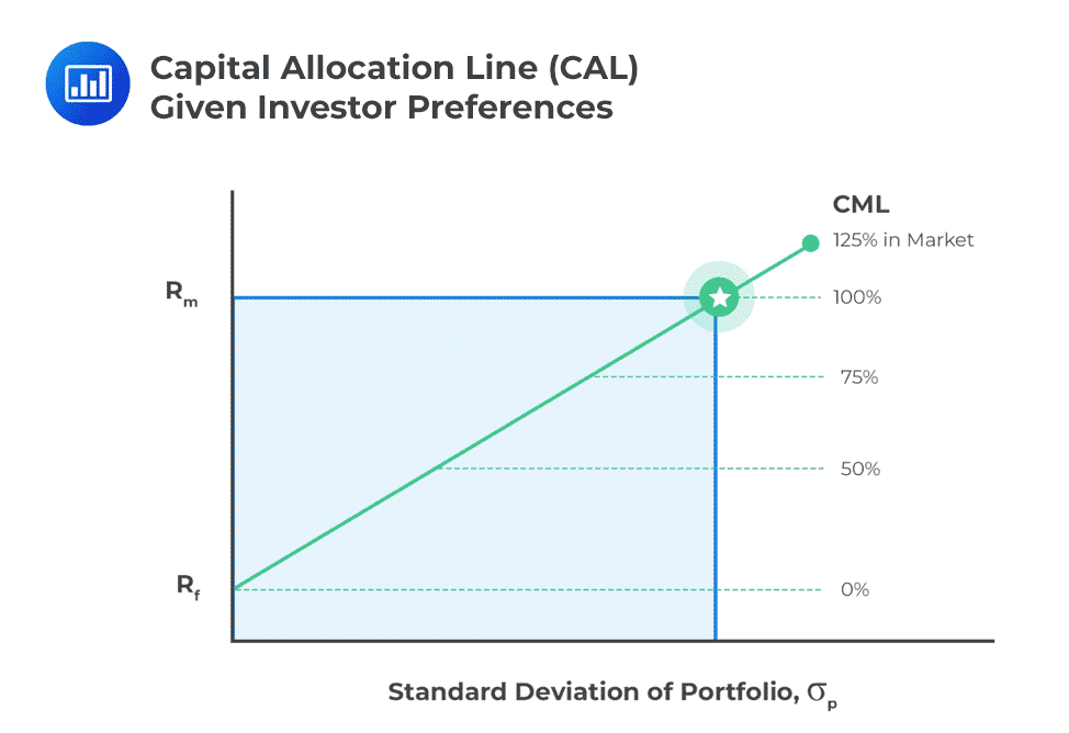The equation can be written as:

$$ E_p=r+\left( \cfrac {E_M-r}{\sigma_M} \right) \sigma_P $$

The factor \(\left( \cfrac {E_M-r}{\sigma_M} \right)\) is usually referred to as the market price of the risk, and on the capital market line, it is equal to the gradient of the line.

We can, therefore, represent the above CML equation in words as:

$$\text{Expected Return}=\text{Risk free rate}+\text{Market price of risk}\times\text{Portfolio Risk}$$

Example: Expected Return using CML

You are given that the market standard deviation is 20%, the risk-free rate is 3%, and the return on the market is 8%.

Calculate the expected return of a portfolio with a portfolio standard deviation of 5%

Solution

From the CML equation, we know that the expected return of a portfolio is given by:

$$ E_p=r+\left( \cfrac {E_M-r}{\sigma_M} \right) \sigma_P $$

Applying the formula, we get:

$$ E_p=0.03+\left( \cfrac {0.08-0.03}{0.2} \right)005 =4.25\% $$

Reduction of Portfolio Risk Through Diversification

It is important to note that the correlation between securities will usually have an impact on the overall variance of the portfolio. In principle, a higher correlation between assets in a portfolio will result in a higher portfolio variance. The inverse is also true.

It is worth noting that the correlation between assets in the portfolio would not generally affect the portfolio’s expected return.

By combining a portfolio of risky assets with a risk-free asset, we can improve the portfolio’s return-risk characteristics, resulting in a better trade-off. This combination is called the capital allocation line, and the proportion of allocation to risky assets versus allocation to the risk-free asset will depend on the investor’s risk preferences.

Recall that:

$$ \sigma^2=Var(R_p )=\sum _{ j }^{ }{ \sum _{ k }^{ }{ { w }_{ j }{ w }_{ k }{ C }_{ jk } } } $$

This can be written as:

$$ \sigma^2=Var(R_p )= \sum _{ \forall j }^{ }{ { w }_{ j }^{ 2 }{ \sigma }_{ j }^{ 2 } } +\sum _{ \forall j }^{ }{ \sum _{ \forall j\neq k }^{ }{ { w }_{ j }{ w }_{ k }{ C }_{ jk } } } $$

You can see this clearly if you consider two assets case. The lower the covariance between the securities, means the lower the variance and hence the risk. This, therefore, implies that the overall risk of the portfolio can be reduced by investing in assets whose returns are uncorrelated or more plainly, independent assets.

Independent here means that the covariance is zero and thus the expression above reduces to :

$$ \sigma_p^2=Var(R_p )=\sum _{ \forall j }^{ }{ { w }_{ j }^{ 2 }{ \sigma }_{ j }^{ 2 } } $$

To understand this more clearly, let us assume that we invest equal amounts of assets. Then,

$$ w_j=\frac {1}{n} $$

So,

$$ \begin{align*} \sigma_p^2 =Var(R_p ) & =\sum _{ \forall j }^{ }{ { w }_{ j }^{ 2 }{ \sigma }_{ j }^{ 2 } } \\ \sum _{ \forall j }^{ }{ { \left( \frac { 1 }{ n } \right) }^{ 2 }{ \sigma }_{ j }^{ 2 } } & =\left( \frac { 1 }{ n } \right) \sum _{ \forall j }^{ }{ { \left( \frac { 1 }{ n } \right) }{ \sigma }_{ j }^{ 2 } } \\ \end{align*} $$

Now let,

$$ \sum _{ \forall j }^{ }{ { \left( \frac { 1 }{ n } \right) }{ \sigma }_{ j }^{ 2 } } =V $$

Note that \(V\) is the mean variance of the assets in the portfolio. Then,

$$ \sigma_p^2=\frac {V}{n} $$

Intuitively, as \(n\) gets larger, the variance tends to zero. In other words, the more independent assets in the portfolio, the lesser the variance and hence the risk. That is to say; risk can be minimized by diversification.

Limitations of the Mean-Variance Framework with Respect to Assumptions about the Return Distributions

MPT has some limitations, with the major one being that MPT tends to ignore the risk that an investor may fail to meet his or her liabilities. This raises the question as to whether the investments are sustainable in contrast to the investor’s liabilities.

The mean-variance framework is unreliable when the assumption of normality is not met. If the return distribution is not symmetric, the standard deviation is not a reliable or relevant measure of probabilities at the extreme ends of the distribution.

The normality assumption is only strictly appropriate in the presence of a zero-skew (symmetric) distribution. If the distribution leans to the left or the right – something that often happens with financial returns – the mean-variance framework churns out misleading estimates of risk.

Other limitations/practical considerations ignored by the MPT include:

• Restrictions on the marketability of assets: The MPT assumes that any quantities of securities/stocks can be bought and sold. This assumption may not hold in practice as different securities will have a minimum order size.
• Ignores taxation and investment costs which may apply in practice.
• Ignores the restrictions that may be imposed by laws or regulations governing the investment markets.
• Does not consider the restrictions imposed on fund managers on the kind of investment decisions they can make.
• Assumes the same time horizon for all investors, and this may not hold in practice.

Despite the above limitations, the MPT continues to be a cornerstone for portfolio managers by applying statistical techniques to portray to investors the benefits of diversification.