


Investment Risk and Project Analysis
After completing this reading, you should be able to: Discuss the advantages and... Read More

After completing this chapter, the Candidate will be able to:
- Explain the properties of the lognormal distribution and its applicability to option pricing.
- Calculate lognormal based probabilities and percentiles for stock prices
- Calculate lognormal based means and variances of stock prices
- Calculate log-normal-based conditional expectations of stock prices given that options expire in the money.
- Explain the Black Scholes formula
- Recognize the assumptions underlying the Black Scholes model
- Estimate a stock’s historical volatility from past stock price data
- Use the Black Scholes formula to value European calls and puts on stocks with no dividends, stock indices with continuous dividends, stocks with discrete dividends, currencies, and futures contracts.
- Generalize the Black Scholes formula to value gap calls, gap puts, exchange options, chooser options, and forward start options.
A random variable \(X\) is said to have a lognormal distribution if its natural log (ln X) is normally distributed. In other words, given a normally distributed random variable \(X\), another random variable \(a\) will be lognormally distributed if:
$$a=e^x$$
Or,
$$x=ln(a)$$
That is,
If \(X\) is lognormally distributed, with the parameters \(\mu\) and \(\sigma\), we can write,
$$ X \sim \log { N\left( \mu,\sigma^2 \right) } $$
The probability distribution function of a log-normally distributed variable is given by:
$$ f(x)=\cfrac {1}{x \sigma \sqrt{2\pi }} e^{-\frac {1}{2} \left( \frac {logX-\mu}{\sigma} \right)^2 } \text { for } 0 < X < \infty $$
The mean and variance of the lognormal distribution are:
$$ E(X)=e^{\mu+\frac {1}{2} \sigma^2 } $$
And
$$ Var(X)=e^{2\mu+\sigma^2 }{(e^{\sigma^2 }-1)} $$
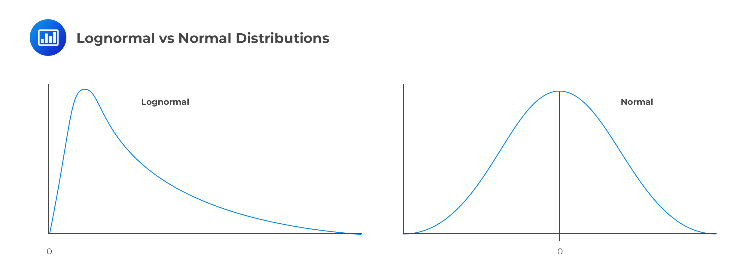
The two most important characteristics of the lognormal distribution are as follows:
These characteristics are in direct contrast to those of the normal distribution, which is symmetrical (zero skews) and can take on both negative and positive values. As a result, the normal distribution cannot be used to model stock prices because stock prices cannot fall below zero. The lognormal distribution is also used to value options.
Recall our definition of a lognormal variable. If \(X\) is normally distributed, the random variable \(a\) is lognormally distributed if the following two conditions hold:
$$a=e^x$$ $$ln{\left(a\right)}=x$$
Starting with the expression \(a=e^x\), we can develop a simple model for the stock price as follows:
$$S_T=S_0e^x$$
In this case, we assume that the variable \(x\) represents the continuously compounded return on the stock from time \(0\) to time \(T\).
Consider the time interval \(t_0,\ t_1,t_2\ldots,t_{n-1},T\) and let the continuously compounded return between time intervals \(t_0\) and \(t_1\) equal to \(r(t_0,t_1)\) and so forth. We assume that the returns between each time interval are independent and identically distributed.
If we split the period \(0\) to \(T\) into n intervals, each of length \(k\) such that \(k=\frac{T}{n}\), then the return from time \(0\) to \(T\) will be equal to:
$$r\left(0,T\right)=r\left(0,k\right)+r\left(k,2k\right)+\ldots+r[\left(n-1\right)k,T]=i=\sum_{i=1}^n{r[i-1k,ik]}$$
Let us assume that the returns \(r[\left(i-1\right)k,ik]\) are normally distributed with mean \(\mu\) and variance \(\sigma^2\). Then, because the returns are independent and identically distributed between each time interval, the mean and variance of the continuously compounded return will be proportionate to time. Hence:
$$E[r\left(0,T\right)]=nμ$$ $$Var\left[r\left(0,T\right)\right]=n\sigma^2$$
Now, define the following:
\(\mu\) = expected return on stock per year;
\(\sigma\) = volatility of the stock price per year;
\(T\) = time in years;
\(\delta\) = dividend yield (of a dividend paying stock);
\(S_T\) = stock price at time T; and
\(S_0\) = stock price at time 0.
We assume that \(\ln{\left(\frac{S_T}{S_0}\right)}\) is normally distributed with mean \((\mu-\frac{\sigma^2}{2})T\) and variance \(\sigma^2T\). Then, for a non-dividend-paying stock:
$$\frac{\ln{S_T}}{\ln{S_0}}\sim \Phi\left[\left(\mu-\frac{\sigma^2}{2}\right)T,\sigma^2T\right]$$
And also
$$\ln{S_T\sim \Phi\left[\ln{S_0+}\left(\mu-\frac{\sigma^2}{2}\right)T,\sigma^2T\right]}$$
The last expression can be written as:
$$\ln{S_T\sim N\left[\ln{S_0+}\left(\mu-\frac{\sigma^2}{2}\right)T,\sigma^2T\right]}\ldots\ldots\ldots\ldots(1)$$
For a dividend-paying stock with a dividend yield of \(\delta\), then (1) becomes:
$$\ln{S_T\sim N\left[\ln{S_0+}\left(\mu-\delta-\frac{\sigma^2}{2}\right)T,\sigma^2T\right]}$$
The subtraction of the dividend yield is necessary since a higher dividend yield means a lower future stock price.
Note: The above relationship holds because mathematically, if \( \ln {x}\) is normally distributed, then \(X\) has a lognormal distribution.
Given a random variable \(X\sim N\left(\mu,\sigma^2\right)\), we can convert this to a standard normal variable \(Z\sim (0,1)\) using the formula below:
$$X=\mu\pm\sigma Z$$
Thus, the lognormal stock price can be given as:
$$\ln{S_T=\left[\ln{S_0+}\left(\mu-\delta-\frac{\sigma^2}{2}\right)T,\sigma\sqrt T Z\right]}$$
Hence:
$$S_T=S_0e^{\left(\mu-\delta-\frac{\sigma^2}{2}\right)\pm\sigma\sqrt T Z}$$
This is the lognormal model for stock prices.
ABC stock has an initial price of $60, an expected annual return of 10%, and annual volatility of 15%.
Calculate the mean and the variance of the distribution of the stock price in six months.
We know that:
$$ \begin{align*} & lnS_T-lnS_0 \sim \Phi \left[ \left( \mu-\frac {\sigma^2}{2}\right)T,\sigma^2 T \right] \\ & =N \left[ln60+ \left(0.10-\frac {0.15^2}{2} \right)0.5,0.15^2×0.5 \right] \\ & \Rightarrow lnS_T \sim N[4.139,0.011] \\ \end{align*} $$
The stock price is lognormally distributed with parameters \(\alpha=4.139\) and \(\sigma=\sqrt{0.011}\).
Sometimes the examiner may want to test your understanding of the lognormal concept by involving confidence intervals.
Since \(ln S_T\) is lognormally distributed, 95% of values will fall within 1.96 standard deviations of the mean. Similarly, 99% of the values will fall within 2.58 standard deviations of the mean.
ABC stock has an initial price of $60, an expected annual return of 10%, and annual volatility of 15%.
Calculate the 99% confidence interval for stock price.
From the previous example, we know that:
$$ \begin{align*} lnS_T & \sim N[4.139,0.011] \\ \end{align*} $$
Recall that the above equation stems from the fact that, given a random variable \(X\sim N\left(\mu,\sigma^2\right)\), can be converted to a standard normal variable \(Z\sim (0,1)\) using the formula below:$$ X=\mu\pm\sigma Z$$
Thus in this we have:
$$\begin{align*}\\ lnS_T & =\mu \pm z_\alpha × \sigma \\ \end{align*}$$
Where:
\(\alpha=0.01\)
\(\sigma=\sqrt {0.011}=0.1049\)
So that:
$$ \begin{align*} & 4.139-z_\alpha×\sigma < lnS_T < 4.139+z_\alpha ×\sigma \\ & \Rightarrow e^{4.139-z_α×σ} < S_T < e^{4.139+z_α×σ} \\ & =e^{4.139-2.58×0.1049} < S_T < e^{4.139+2.58×0.1049} \\ & =47.86 < S_T < 82.24 \\ \end{align*} $$
Therefore, we are 99% sure that in six months’ time, the stock price will be between $47.86 and $82.24.
Since \(S_t\) is lognormally distributed, we can also calculate the probability that an option will expire in the money and its corresponding expected stock price.
Let the current stock price be \(S_0\). We want to answer the following question:
What is the probability that \(S_t < X\) or equivalently \(lnS_t < lnX \) where \(X\) is an arbitrary number?
Now using the formulation,
$$ lnS_T \sim N \left[lnS_0+ \left(\mu-\delta-\frac {\sigma^2}{2} \right) T,\sigma^2 T \right] $$
We can construct a standard normal variable Z (just like normal distribution) as:
$$ Z=\cfrac {lnS_T-lnS_0-\left(\mu-\delta-\frac {\sigma^2}{2} \right) T, T }{\sigma \sqrt {T}} $$
Now consider \(Pr(S_t < X)=Pr(ln S_t < ln X) \).
Subtracting the mean from both \(lnS_t\) and \(ln X\) and dividing by the standard deviation, we have:
$$ Pr(S_t < X)=Pr \left[ \cfrac {lnS_T-lnS_0-\left(\mu-\delta-\frac {\sigma^2}{2} \right) T }{\sigma \sqrt {T}} < \cfrac {lnX-lnS_0-\left(\mu-\delta-\frac {\sigma^2}{2} \right) T }{\sigma \sqrt {T}} \right] $$
But the left-hand side of the inequality is a standard normal random variable. Therefore:
$$ Pr(S_t < X)=Pr \left[ Z < \cfrac {lnX-lnS_0-\left(\mu-\delta-\frac {\sigma^2}{2} \right) T }{\sigma \sqrt {T}} \right] $$
But \(Z \sim N(0,1)\) which implies that:
$$ Pr(S_t < X)=N \left[\cfrac {lnX-lnS_0-\left(\mu-\delta-\frac {\sigma^2}{2} \right) T }{\sigma \sqrt {T}} \right]=N(-d_2) $$
\(d_2\) is the standard Black-Scholes variable with the risk-free rate, \(r\), replaced with the actual expected return on the stock \(\mu\). We will explore the Black-Scholes formula in the next few sections.
Also, we have:
$$ Pr(S_t > X)=1-Pr(S_t < X)=N(d_2) $$
The current price of a non-dividend-paying stock is $50. The stock prices are log-normally distributed with parameters \(\mu=0.075\) and \(\sigma^2=0.25\). An investor has purchased a one-year call option on this stock with a strike price of $55.
Calculate the probability that the call will expire worthless.
The call will expire worthless if the stock price in one year will be less than $55.
We are therefore interested in the probability that:
$$\begin{align}P\left(S_T<55\right)&=P\left[\ln{\left(S_T\right)}<\ln{\left(\frac{55}{50}\right)}\right]\\ &=\phi\left(\frac{\ln{\left(1.1\right)}-(0.075-0.25\times0.5)}{\sqrt{0.25}}\right)\\ &=\phi\left(0.29\right)=0.61409 \end{align}$$
The lognormal model for a stock price is given as:
$$S_T=S_0e^{\left(\mu-\delta-\frac{\sigma^2}{2}\right)T+\sigma\sqrt T Z} $$
We know that \(\ln{S_T}\) is normally distributed with mean \(\ln{S_0+}\left(\mu-\delta-\frac{\sigma^2}{2}\right)T\) and standard deviation, \(\sigma\sqrt T\).
\(S_T\) is, therefore, log normally distributed.
Our interest may therefore be to find the expected value and variance of \(S_T\).
$$S_T=S_0e^{\left(\mu-\delta-\frac{\sigma^2}{2}\right)T+\sigma\sqrt T Z}$$
For a dividend paying stock with a continuous dividend yield, \(\delta\), the expected stock price is given as: $${E(S}_T)=S_0e^{\left(\mu-\delta-\frac{\sigma^2}{2}\right)T+\frac{1}{2}\sigma^2T}=S_0e^{\left(u-\delta\right)T}$$
For a non-dividend-paying stock, the formula simplifies to:
$$ E\left(S_T\right)=S_0e^{\mu T} $$
For a dividend-paying stock with a continuous dividend yield \(\delta\), the variance of the stock price is given as:
$$Var\left(S_T\right)=S_0^2e^{2\left(\mu-\delta\right)T}(e^{\sigma^2T}-1)$$
For a non-dividend-paying stock, the formula simplifies to:
$$Var\left(S_T\right)=S_0^2e^{2\mu T}(e^{\sigma^2T}-1)$$
The current price of a non-dividend-paying stock is $90. The expected return on the stock and annual volatility is 20% and 15%, respectively.
Calculate the one-year expected stock price and variance of the stock price.
The expected stock price is given by:
$$E\left(S_T\right)=S_0e^{\mu T}$$
In this case, we have:
\(S_0=90, \mu=20\% , \sigma=15\%\) and \(T=1\) so that:
$$E\left(S_T\right)=90e^{0.2\times1}=$109.93$$
The variance of the stock price is given by:
$$Var\left(S_T\right)=S_0^2e^{2\mu T}(e^{\sigma^2T}-1)={90}^2e^{2\times0.2}\left(e^{{0.15}^2}-1\right)=\$274.97$$
The conditional expectation of a random variable, say \(X\), given \(Y\) is denoted as \(E(X|Y)\). For a discrete distribution:
$$E\left(X\middle| Y=y\right)=\sum_{i}{x_iP\left(X=x_i\middle| Y=y\right)=\sum_{i}{x_i\frac{P(X=x,Y=y)}{P(Y=y)}}}$$
For a continuous distribution:
$$E\left(X\middle| Y=y\right)=\int_{x}^{\infty}{xf\left(x\middle| y\right)dx=}\int_{x}^{\infty}{x\frac{f(x,y)}{f(y)}dx}$$
$$E\left(X\middle| Y=y\right)=\int_{x}^{\infty}{xf\left(x\middle| y\right)dx=}\int_{x}^{\infty}{x\frac{f(x,y)}{f(y)}dx}$$
When considering options on an underlying stock, it may be of interest to determine the expected stock price given the option expires in the money.
Given \(S_T\) as the stock price and \(K\) as the strike price of say a put option, we are interested in computing \(E(S_T|S_T<K)\). This is the expected stock price conditional on \(S_T<K\). We need to calculate:
$$E\left(S_T\middle| S_T<X\right)$$
To do this, we need to include only the proportion density representing stock rises above \(X\), the strike price.
From a given binomial model, the stock price at expiration can be $30, $50, $70, or $90, with probabilities \(\frac{1}{8},\frac{3}{8},\frac{3}{8}\), and \(\frac{1}{8}\). A put option has been written on this underlying stock with a strike price of $60.
Calculate the expected stock price conditional on the option expiring in the money.
Our task is to compute:
$$E(S_T|S_T\lt X)$$
We first compute the partial expectation, which is given by:
$$ Pr(S_t < 60)=\sum _{ { S }_{ t } < 60 }^{ }{ Pr\left( S_{ t } \right) \times S_{ t }=\frac { 1 }{ 8 } \times 30+\frac { 3 }{ 8 } \times 50=$22.50 } $$
You must realize that $22.50 is not the actual stock price expectation since it is even lower than the lowest possible price ($30), and hence it is called partial expectation.
The partial expectation of $22.5 is lower than the lowest possible stock price. We need to compute the conditional expectation, where the condition \(S_t < \$50\), happens with probability \(\frac{1}{8}+\frac{3}{8}=\frac{1}{2}\).
To convert a partial expectation into a conditional expectation, we divide it by the probability of the conditioning event (in this case \(S_t < 60\)). That is:
$$ E(S_t│S_t < 60)=\cfrac {1}{Pr(S_t < 60)} \sum _{ { S }_{ t } < 60 }^{ }{ Pr\left( S_{ t } \right) \times S_{ t }=\frac{1}{0.5}\times \left[ \frac { 1 }{ 8 } \times 30+\frac { 3 }{ 8 } \times 50 \right]=2 \times \$22.50=\$45}$$
We transfer the same analogy to lognormal distribution, where we will use integral instead of summation.
The partial expectation of \(S_t\) conditional on \(S_t < X\) is:
$$ \begin{align*} E\left(S_t\middle| S_t<X\right)&=\int _{ 0 }^{ X }{ { S }_{ t }f\left( { S }_{ t };{ S }_{ 0 } \right) d{ S }_{ t } }\\ &={ S }_{ 0 }{ e }^{ \left( \mu -\delta \right) t }N\left( \cfrac { lnX-\left[ lnS_{ 0 }+\left( \mu -\delta -\frac { \sigma ^{ 2 } }{ 2 } \right) T \right] }{ \sigma \sqrt { T } } \right) \\ & =S_0 e^{(\mu-\delta)t} N(-d_1 ) \\ \end{align*} $$
Where:
\(f(S_t;S_0)\) is the probability density of \(S_t\) conditional on \(S_0\), and
\(d_1\) is the Black-Scholes \(d_1\) where \(\mu\) has replaced \(r\).
Recall that,
$$ \begin{align*} & Pr(S_t < X)=N(-d_2) \\ \Rightarrow & E(S_t│S_t < X) =S_0 e^{(\alpha-\delta)t} \cfrac { N(-d_1 )}{N(-d_2 ) } \\ \end{align*} $$
Note that we are still dealing with the put option above! For a call option, we need:
$$ \begin{align*} & =\int _{ 0 }^{ X }{ { S }_{ t }f\left( { S }_{ t };{ S }_{ 0 } \right) d{ S }_{ t } } ={ S }_{ 0 }{ e }^{ \left( \mu -\delta \right) t }N\left( \cfrac { lnS_{ 0 }-\left[ lnX+\left( \mu -\delta -\frac { \sigma ^{ 2 } }{ 2 } \right) T \right] }{ \sigma \sqrt { T } } \right) \\ & =S_0 e^{(\mu-\delta)t} N(d_1) \\ \end{align*} $$
And using the same analogy as a put option, we have:
$$ E(S_t│S_t>X) =S_0 e^{(\alpha-\delta) t} \cfrac {N(d_1 )}{N(d_2 ) } $$
Lastly, the formulas above adjust accordingly when in the case of non-dividend stock, that is: \(\delta=0\).
A one-year European call option has been issued on a stock whose returns are normally distributed with mean and variance of 10% and 25%, respectively. The stock pays continuous dividends at the rate of 2% p.a. The current stock price is $70, and the strike price of the call is $72. On maturity, the stock was trading at $75.
Calculate the expected stock price conditional on the option expiring in the money.
We need to calculate:
$$E\left(S_T\middle| S_T>X\right){=S}_0e^{\left(\alpha-\delta\right)T}\frac{N\left(d_1\right)}{N\left(d_2\right)\ }$$
Where:
$$N\left(d_1\right)=N\left(\frac{ln\ S_0\ {-\ln{X+\left(\alpha-\delta-\frac{\sigma^2}{2}\right)T}}}{\sigma\sqrt T}\right)=N\left(\frac{\ln{\left(\frac{70}{72}\right)}+\left(0.1-0.02-\frac{0.25}{2}\right)}{0.25}\right)=N(-0.293)$$
$$N\left(d_2\right)=N\left(\frac{ln\ S_0\ {-\ln{S_T+\left(\mu-\delta-\frac{\sigma^2}{2}\right)T}}}{\sigma\sqrt T}\right)=\left(\frac{\ln{\left(\frac{70}{75}\right)}+\left(0.1-0.02-\frac{0.25}{2}\right)}{0.25}\right)=N(-0.456)$$
We read the values of \(d_1\) and \(d_2\) from the standard normal tables. Thus,
$$E\left(S_T\middle| S_T>72\right)=70e^{\left(0.1-0.02\right)}\frac{1-0.61409}{1-0.67724}=\$90.67$$
The Black-Scholes-Merton model is used to price European options and is undoubtedly the single most important tool for analyzing derivatives.
For a standard European call option, the formula is given as:
$$C=SN\left(d_1\right)-Ke^{-rt}N(d_2)$$
For a standard European put option, the formula is given as:
$$P=Ke^{-rt}N\left({-d}_2\right)-SN(-d_1)$$
Where:
\(S\) = price of the underlying security.
\(K\)= strike price of the call or the put.
\(r\) = risk-free rate of return.
\(d_1\) and \(d_2\) are as defined in the previous section with \(\alpha\) replaced with the risk-free rate \(r\).
\(N(x)\) = probability that a variable with a standard normal distribution will be less than 1.
The model takes into account the fact that the investor has the option of investing in an asset earning the risk-free interest rate. The overriding argument is that the option price is purely a function of the volatility of the stock’s price (option premium increases as volatility increases.)
A stock’s historical volatility refers to the volatility obtained from historical stock returns. Historical volatility can be computed from stock price data recorded at specified intervals, say daily, by computing the standard deviation of the continuously compounded returns per day.
Consider a daily time interval and let \(S_i\) represent the recorded stock price at the end of day \(i\) and \(\mu_i\) the continuously compounded return for day \(i\).
Then, the continuously compounded return for day \(i\) is calculated as:
$$\mu_i=ln\left(\frac{S_i}{S_{i-1}}\right)$$
The volatility of the continuously compounded returns is computed as the square root of the variance of the stock returns.
For a given set of historical stock price data, the variance of the stock returns, \(\sigma^2\), is given as:
$$\sigma^2=\frac{\sum_{i=1}^{n}{(\mu_i^2-\bar{\mu}\ )}}{n-1}$$
Where \(n\) represents the number of entries and \(\bar{u}\) the mean of the daily returns and is computed as:
$$\bar{\mu}=\frac{\sum_{i=1}^{n}\mu_i}{n}$$
The formula for the variance of stock returns can be written as:
$$\sigma^2=\frac{\sum_{i=1}^{n}\mu_i^2}{n-1}-\frac{\sum_{i=1}^{n}u_i}{n(n-1)}$$
The historical volatility \(\sigma\) is then obtained by taking the square root of the variance.
$$\sigma=\sqrt{\frac{\sum_{i=1}^{n}\mu_i^2}{n-1}-\frac{\sum_{i=1}^{n}u_i}{n(n-1)}}$$
The volatility of short time periods can be scaled to give the volatility of longer time periods. For example, to convert daily volatility to annual volatility, we use the following formula:
$$\text{Annual Volatility}=\text{daily volatility}\times \sqrt{\text{Number of days in a year}}$$
Intuitively, it can be seen that:
$$\text{Annual Volatility}=\text{Monthly Volatility}\times \sqrt{\text{Number of months in a year}}$$
Conversely,
$$\text{Daily Volatility} =\frac{\text{Annual Volatility}}{\sqrt{\text{Number of days in a year}}}$$
And,
$$\text{Monthly volatility}= \frac{\text{Annual volatility}}{\text{Number of months in a year}}$$
The following table shows the stock price of a Kayak Group.
$$ \begin{array}{l|c|c|c|c|c|c} \text{Day}_i & 0 & 1 & 2 & 3 & 4 & 5 \\ \hline \text{Stock Price }S_i & 55.5 & 53.2 & 54.3 & 57.1 & 55.7 & 52.9 \\ \end{array} $$
Estimate the volatility per day of the stock based on the data.
We use the following table to calculate the estimate of the standard deviation of the daily return.
$$ \begin{array}{l|c|c|c|c|c|c} \text{Day}_i & 0 & 1 & 2 & 3 & 4 & 5 \\ \hline \text{Stock Price }S_i & 55.5 & 53.2 & 54.3 & 57.1 & 55.7 & 52.9 \\ \hline \text{Price Relative } \frac{S_i}{S_{i-1}} & \text{} & 0.95856 & 1.020676 & 1.051565 & 0.97548 & 0.9497 \\ \hline \text{Daily Return } \mu_i=ln \left(\frac {S_i}{S_{i-1}} \right) & \text{} & -0.04232 & 0.020466 & 0.05028 & -0.02482 & -0.05158 \\ \hline \mu_i^2 & \text{} & 0.001791 & 0.000419 & 0.002528 & 0.000616 & 0.00266 \\ \hline \end{array} $$
To estimate the standard deviation of the daily return, we need the following inputs:
$$ \sum_{i=1}^{n}u_i=-0.04798$$
$$\sum_{i=1}^{n}u_i^2=0.008014688$$
So that the standard deviation of the daily return is given by:
$$\sigma^2=\frac{\sum_{i=1}^{n}\mu_i^2}{n-1}-\frac{\sum_{i=1}^{n}u_i}{n(n-1)}=\sqrt{\frac{0.008014688}{4}-\frac{{-0.04798}^2}{5\times4}}=0.04346$$
Thus, the volatility per annum is:
$$0.04346 \times \sqrt{252} =0.6898692 \approx 69\%$$
The value of a call option is given by:
$$ C_0=S_0×N(d_1)–Ke^{-rT}×N(d_2) $$
The value of a put option is given by:
$$ p_0=Ke^{-rT}×N(-d_2 )-S_0×N(-d_1) $$
Where:
$$ \begin{align*} d_1 & =\cfrac {ln\frac {S_0}{K}+ \left[r-\delta+\left(\frac {\sigma^2}{2} \right) \right]T}{\sigma \sqrt {T}} \\ d_2 & =d_1-({\sigma \sqrt {T}}) \\ \end{align*} $$
Where:
\(T\) = time to maturity, assuming 365 days per year;
\(S_0\) = asset price;
\(K\) = exercise price;
\(r\) = continuously compounded risk-free rate;
\(\sigma\) = volatility of continuously compounded returns on the stock;
\(\delta\) = continuous dividend yield; and
\(N(d_i )\) = cumulative distribution function for a standardized normal distribution variable.
You are given that \(S_0 = $100\), \(K = $90\), \(T = 6 \text{ months}\), \(r = 10\%\), and \(\sigma = 25\%\).
Calculate the value of a call option.
We know that:
$$ C_0=S_0×N(d_1)–Ke^{-rT}×N(d_2) $$
And
$$ \begin{align*} d_1 & =\cfrac {ln\frac {S_0}{K}+ \left[r+\left(\frac {\sigma^2}{2} \right) \right]T}{\sigma \sqrt {T}} \\ & = \cfrac {ln\frac {100}{90}+\left[0.10+ \left(\frac {0.25^2}{2} \right) \right]0.5}{0.25 \sqrt {0.5}}=0.9672 \\ d_2 & =d_1-({\sigma \sqrt {T}}) \\ & =0.9672-({0.25 \sqrt {0.5}})=0.7904 \\ \end{align*} $$
From the normal tables,
$$ N(0.97)=0.8333 \text { and } N(0.79)=0.7852 $$
Then,
$$ C_0=100×N(0.9672)–90e^{-0.10×0.50}×N(0.7904)=$16.11 $$
Note that the intrinsic value of the option is $10 – our answer must be at least that amount.
Assume that we have a known dividend \(d\) distributed a time \(T_1 < T\), where \(T\) is the maturity date. To value calls and puts when there are such dividends, we modify the BSM model by replacing \(S_0\) with \(S\), where:
$$ S=S_0-D $$
Where \(D\) is the sum of the present value discounted at the risk-free rate of interest \(r\) of the dividend payments during the life of the option.
For example, with dividends \(D_1\) and \(D_2\) at times \(\Delta t_1\) and \(\Delta t_2\), then:
$$ S=S_0-D_1 e^{r \frac {\Delta t_1}{m}}-D_2 e^{r \frac {\Delta t_2}{m}} $$
\(\Delta t_i\) represents the amount of time until the ex-dividend date.
\(m\) is a division factor to bring the \(\Delta t\) to a full year. For example, if \(\Delta t= 2\ \text{months}\), and \(m= 12\) then, \(\frac{\Delta t}{m}=\frac{2}{12}=0.1667\ \text{years}\).
For example, if \(\Delta t\)= 2 months, and \(m\)= 12 then, \(\frac {\Delta t}{m}=\frac {2}{12}=0.1667 \text{ years}\).
After this, it is important to note everything else in the computational formulas remains the same as before. That is:
The value of a call option is given by:
$$ C_0=S×N(d_1)–Ke^{-rT}×N(d_2) $$
The value of a put option is given by:
$$ p_0=Ke^{-rT}×(1-N(d_2 ))-S×(1-N(d_1 )) $$
Where
$$ \begin{align*} d_1 & =\cfrac {ln \frac {S}{K}+ \left[r+\left(\frac {\sigma^2}{2} \right) \right]T}{\sigma \sqrt {T}} \\ d_2 & =d_1-({\sigma \sqrt {T}}) \\ \end{align*} $$
\(S\) is simply \(S_0\) adjusted to include dividends payable.
The underlying argument here is that on the ex-dividend dates, the stock prices are expected to reduce by the amounts of the dividend payments.
A one-year European call option has been written on a stock paying dividends. The stock pays half-yearly dividends, and a dividend of $0.20 per share has just been paid. Subsequent dividends are expected to increase by $0.05 each.
The following additional information is given:
Calculate the price of a one-year call option on this stock.
The present value of the dividend payments is:
$$=0.25e^{-0.03\times0.5}+{0.3e}^{-0.03}=$0.54$$
Next, we compute the value of \(S\),
$$S=S_0-D=72-0.54=$71.46$$
The price of a call is given by:
$$C_0=S\times N(d_1)–Ke-rT×N(d2)$$
Where:
$$d_1=\frac{\ln{\frac{S}{K}+\left[r+\left(\frac{\sigma^2}{2}\right)\right]T}}{\sigma\sqrt T}=\frac{\ln{\frac{71.46}{80}+\left[0.03+\left(\frac{{0.3}^2}{2}\right)\right]}}{0.3}=-0.1263$$
$$d_2=d_1-(\sigma\sqrt T)=-0.1263-0.3=-0.4263$$
Thus:
$$\begin{align}C_0&=71.46\times N\left(-0.1263\right)-80e^{-0.03}\times N\left(-0.4263\right)\\ &= 71.46\left(1-0.5503\right)-80\left(1-0.6651\right)=5.343562\end{align}$$
In case of continuously paid dividends at a rate of \(q\), you are still expected to replace \(S_0\) with \(S\), where:
$$ S=S_0e^{-qT} $$
The value of a call option is given by:
$$ C_0=S_0 e^{-qT}×N(d_1)–Ke^{-rT}×N(d_2) $$
The value of a put option is given by:
$$ p_0=Ke^{-rT}×N(-d_2 )-S_0 e^{-qT}×N(-d_1) $$
Where:
$$ \begin{align*} d_1 & =\cfrac {ln\frac{S_0}{K}+ \left[r-q+\left(\frac {\sigma^2}{2} \right) \right]T}{\sigma \sqrt {T}} \\ d_2 & =d_1-({\sigma \sqrt {T}}) \\ \end{align*} $$
Where all parameters are defined as before. One more thing to note, in the formulas above, we have taken \(S_0\) but it can be the stock price at any time \(t\), \(S_t\). In this case, our length of time will be \((T-t)\) while other things remain the same.
A 3-month put option has been written on a stock. The stock is currently priced at $50 and pays continuous dividends at 3% per annum. The continuously compounded risk-free rate of return is 10% per annum, and the volatility is 20% per annum. We are given that the exercise price of the put is $45.
Calculate the price of this option.
We know that:
$$p_0=Ke^{-rT}\times N\left(-d_2\right)-S_0e^{-qT}\times N({-d}_1)$$
Where:
$$d_1=\frac{\ln{(\frac{50}{45})+\left[0.1-0.03+\left(\frac{{0.2}^2}{2}\right)\right]0.25}}{0.2\sqrt{0.25}}=1.2786$$
$$d_2=d_1-(\sigma\sqrt T)=1.2786-0.2\sqrt{0.25}=1.1786$$
Thus,
$$\begin{align}p_0&=45e^{-0.1\times0.25}N\left(-1.18\right)-50e^{0.03\times0.25}\times N(-1.28)\\&=45e^{-0.1\times 0.25}\left(1-0.8810\right)-50e^{0.03\times 0.25}\times \left(1-0.8997\right)=\$0.17\end{align}$$
The price of a currency option is evaluated by replacing the dividend yield with the foreign interest rate \(r_c\) in the formula for \(d_1\).
Currency options usually involve a spot exchange rate is \(x\), which is normally expressed as the domestic currency per unit of foreign currency, and the foreign interest rate \(r_c\). The valuation of European options on currency using Black-Scholes is:
$$ c=xe^{(-r_cT)}N\left(d_1\right)-Ke^{\left(-rT\right)}N(d_2)(\text{European Call options}) $$
$$ p=Ke^{\left(-rT\right)}N\left(-d_2\right)-xe^{(-r_cT)}N\left({-d}_1\right)(\text{European Put options)} $$
Where:
$$d_1=\frac{ln\frac{x}{K}+\left(r-r_c+\frac{1}{2}\sigma^2\right)T}{\sigma\sqrt T}$$
And
$$ d_2=d_1-\sigma\sqrt T$$
A 6-month dollar-denominated European call option on Canadian Dollars has been purchased.
The following information is given about the call:
Calculate the price of the call option.
The price is given by:
$$ c=xe^{(-r_cT)}N\left(d_1\right)-Ke^{\left(-rT\right)}N(d_2) $$
Where:
$$\begin{align}d_1&=\frac{ln\frac{x}{K}+\left(r-r_c+\frac{1}{2}\sigma^2\right)T}{\sigma\sqrt T}\\ &=\frac{\ln{\left(\frac{0.78}{0.75}\right)}+\left(0.04-0.06+0.5\times{0.2}^2\right)0.5\ }{0.2\sqrt{0.5}}=0.277 \end{align}$$
Also,
$$d_2=d_1-\sigma\sqrt T=0.277-0.2\sqrt{0.5}=0.1359$$
Thus,
$$\begin{align}c_0&=0.78e^{(-0.06\times0.5)}\times N\left(0.28\right)-0.75e^{-0.04\times0.5}N\left(0.14\right)\\&=0.757\times0.61026-0.73515\times0.55567=\$0.0534\end{align}$$
Recall that for a dividend paying stock,
$$d_{1}=\frac{\ln (S / K)+\left(r-\delta+\frac{1}{2} \sigma^{2}\right) T}{\sigma \sqrt{T}}$$
We price a European option on a futures contract by using the future price as the stock price, and by setting the dividend yield equal to the risk-free rate. Thus, the resulting formula is:
$$ \begin{align*} p& =Ke^{-rT} N(-d_1 )-Fe^{-rT} N(-d_2 ) \\ c & =Fe^{-rT} N(d_1 )-Ke^{-rT} N(d_2) \\ \end{align*} $$
Where:
$$ \begin{align*} d_1 &=\cfrac {ln \frac {F_0}{K}+\left[\frac {\sigma^2}{2} \right]T }{\sigma \sqrt {T}} \\ d_2 & =d_1-{\sigma \sqrt {T}} \\ \end{align*} $$
Again, we can use put-call parity.
The current price of futures is $70, and bearing volatility is 20%. The risk-free rate of return is 6% per year.
Calculate the 5-month European put on the futures with a strike price of $65.
We know that:
$$p=Ke^{-rT}N\left(-d_2\right)-Fe^{-rT}N(-d_1)$$
Where:
$$d_1=\frac{\ln{\frac{F_0}{K}+\left[\left(\frac{\sigma^2}{2}\right)\right]T}}{\sigma\sqrt T}=\frac{\ln{\frac{70}{65}+\left(\left(\frac{{0.2}^2}{2}\right)\right)\ \frac{5}{12}}}{0.2\sqrt{\frac{5}{12}}}=0.6386$$
$$d_2=0.6386-0.2\sqrt{\frac{5}{12}}=0.5095$$
Therefore,
$$\begin{align} p&=e^{-0.06\times\frac{5}{12}}\left(65N\left(-0.5095\right)-70N\left(-0.6386\right)\right)\\ &=e^{-0.06\times\frac{5}{12}}\left(65\times(1-0.6962 )-70\times(1-0.7385)\right)= 1.4064 \end{align}$$
A gap option has a strike price, \(K_1\), and a trigger price, \(K_2\). The trigger price determines whether or not the option will have a nonzero payoff. The strike price determines the actual amount of the payoff.
For a gap call option, the payoff will always be nonzero (positive or negative) as long as the final stock price exceeds the trigger price. For a gap put option, the payoff will always be nonzero as long as the final stock price is less than the trigger price. If \(K_1=K_2\), the gap option payoff will be the same as that of an ordinary option.
When \(K_2>K_1\),
$$ \text{Gap call option payoff}=\begin{cases} S_{ T }-K_{ 1 } & \text{if }S_{ T }>K_{ 2 } \\ 0, & \text{if }S_{ T }\le K_{ 2 } \end{cases} $$
Where:
\(K_1\) = strike price; and
\(K_2\) = trigger price.
If the trigger price is less than the strike price for a gap call option, negative payoffs are possible.
A modified Black-Scholes formula for the gap option is as below:
For a gap call:
$$ C(S,K_1,K_2,\sigma,r,T,\delta) = Se^{-δT} N(d_1) – K_1 e^{-rT} N(d_2) $$
Where,
$$ d_1 =\cfrac { ln\left[ \frac {Se^{-\delta T} }{ K_2 e^{-r T } } \right]+\frac {1}{2} \sigma^2 T }{\sigma \sqrt{T} }$$
Alternatively,
$$d_1=\frac{\ln{\left(\frac{S}{K_2}\right)}+\left(r-\delta+\frac{\sigma^2}{2}\right)T}{\sigma\sqrt T}$$
And,
$$d_2 = d_1-{\sigma \sqrt{T} } $$
The price of the above gap call is greater than the price given by the Black–Scholes–Merton formula for a regular call option with a strike price \(K_2\) by:
$$\left(K_2-K_1\right)e^{-rT}N\left(d_2\right)$$
For a gap put:
$$ P(S,K_1,K_2,\sigma,r,T,\delta)= K_1 e^{-rT} N(-d_2 )-Se^{-\delta T} N(-d_1) $$
Where,
$$ \begin{align*} d_1 & =\cfrac { ln\left[ \frac {Se^{-\delta T} }{ K_2 e^{-r T } } \right]+\frac {1}{2} \sigma^2 T }{\sigma \sqrt{T} } \\ \text{And},& \\ d_2 &= d_1-{\sigma \sqrt{T} } \\ \end{align*} $$
A gap call on company A’s stock bears a strike price of $55 and a trigger price of $60 with an expiration period of 2 years. The stock price is currently $58 per share with dividends paid at a continuously compounded rate of interest of 3%. The risk-free rate of interest is 9% and price volatility is 33%.
Calculate the price of the gap option.
We know that for a gap call:
$$ C(S,K_1,K_2,\sigma,r,T,\delta) = Se^{-\delta T} N(d_1) – K_1 e^{-rT} N(d_2) $$
Where,
$$\begin{align*} d_1 & =\cfrac { ln\left[ \frac {Se^{-\delta T} }{ K_2e^{-r T) } } \right]+\frac {1}{2} \sigma^2 T }{\sigma \sqrt{T} } \\ \text{And}, & \\ d_2 &= d_1-{\sigma \sqrt{T} } \\ d_1 & = \cfrac {ln \left[\frac {58e^{-0.03×2}}{60e^{-0.09×2} } \right]+\frac {1}{2} ×0.33^2×2}{0.33 \sqrt{2}} =0.41783 \\ d_2 & = 0.41783 – 0.33 \sqrt {2}=-0.048858 \\ \Rightarrow C(S,K_1,K_2,\sigma,r,T,\delta) & = 58e^{-0.03×2} N(0.41783) – 55e^{-0.09×2} N(-0.048858) \\ & =58e^{-0.03×2}\:\left(0.6620\right)\:-\:55e^{-0.09×2}\:\left(1-0.5195\right)=14.08588\approx 14.09 \\ \end{align*}$$
These options are also called out-performance options. An exchange option is characterized by the fact that its payoff is determined by a benchmark asset, in that it should outperform the asset. The payoff of this option can be stated as:
$$ \text{max}(0,S_T-X_T) $$
Where:
\(T\) = option’s time to expiration;
\(S_T\) = the price of the underlying asset; and
\(X_T\) = price of the benchmark asset at time \(T\).
The price of the European exchange can be generalized by the Black-Scholes formula given by:
$$ C(S,X,\sigma,\delta_s,\delta_X,T)=Se^{-(\delta_s )T} N(d_1 )-Xe^{-(\delta_X )T} N(d_2) $$
Where:
$$ \begin{align*} d_1 & =\cfrac { ln\left( \frac {Se^{-(\delta_s T)} }{ Ke^{-(\delta_K T) } } \right)+\frac {1}{2} \sigma^2 T }{\sigma \sqrt{T} } \\ d_2 &= d_1-{\sigma \sqrt{T} } \\ \sigma & =\sqrt { \sigma_s^2+\sigma_X^2-2\rho \sigma_S \sigma_X ) } \\ \end{align*} $$
The variables are defined as below:
\(\delta_X\) = the yearly continuously compounded dividend yield on the benchmark asset;
\(\delta_S\) = the yearly continuously compounded dividend yield on the underlying asset;
\(\rho\) = the correlation coefficient between returns on the two assets;
\(\sigma_X\) = the annual price volatility of the benchmark asset; and
\(\sigma_S\) = the annual price volatility of the underlying asset.
One share of Company A is used as the underlying asset on an exchange option which is currently priced at $320 per share. One share of Company B is used as the benchmark asset, whose shares are priced at $300 per share. Company A’s annual volatility is 0.34 and pays annual dividends at a compound rate of 20% while that of Company B’s annual volatility is 0.60 and pays annual dividends at a rate of 2% compounded yearly.
The correlation coefficient between the companies’ compounded returns is 0.84, and the option expires in 5 years.
Calculate the price of this option.
We know that:
$$ (S,X,\sigma,\delta_s,\delta_X,T)=Se^{-(\delta_s )T} N(d_1 )-Xe^{-(\delta_X )T} N(d_2) $$
Where:
$$ \begin{align*} d_1 & =\cfrac { ln\left( \frac {Se^{-(\delta_s T)} }{ Ke^{-(\delta_K T) } } \right)+\frac {1}{2} \sigma^2 T }{\sigma \sqrt{T} } \\ d_2 &= d_1-{\sigma \sqrt{T} } \\ \sigma & =\sqrt { \sigma_s^2+\sigma_X^2-2\rho \sigma_S \sigma_X ) } \\ \end{align*} $$
Where,
\(\delta_X\) = the yearly continuously compounded dividend yield on the benchmark asset;
\(\delta_S\) = the yearly continuously compounded dividend yield on the underlying asset;
\(\rho\) = the correlation coefficient between returns on the two assets;
\(\sigma_X\) = the annual price volatility of the benchmark asset; and
\(\sigma_S\) = the annual price volatility of the underlying asset.
Now,
$$ \begin{align*} \sigma & =\sqrt { \sigma_s^2+\sigma_X^2-2\rho \sigma_S \sigma_X ) } \\ &=\sqrt { 0.34^2 +0.60^2-2×0.84×0.34×0.60 }=0.36453 \\ \end{align*} $$
Also,
$$ \begin{align*} d_1 & =\cfrac { ln\left( \frac {Se^{-(\delta_s T)} }{ Ke^{-(\delta_K T) } } \right)+\frac {1}{2} \sigma^2 T }{\sigma \sqrt{T} } \\ & = \cfrac {ln \left( \frac {320e^{-0.20×5}}{300e^{-0.02×5} } \right)+\frac {1}{2}×0.36453^2×5}{0.36453 \sqrt{5}}=-0.617406 \\ d_2 &= d_1-{\sigma \sqrt{T} } \\ & = -0.617406-0.36453 \sqrt {5}=-1.432520 \\ \end{align*} $$
Therefore,
$$ \begin{align*} (S,X,\sigma,\delta_s,\delta_X,T) & =Se^{-(\delta_s )T} N(d_1 )-Xe^{-(\delta_X )T} N(d_2) \\ & =320e^{-0.20×5} N(-0.617406)-300e^{-0.02×5} N(-1.432520) \\ & =31.5058-20.728=10.7778 \approx 10.98 \\ \end{align*} $$
Also called often called an “as you like it option,” this is a type of exotic option where after some predetermined time, the holder can choose whether the option is a call or a put. For instance, assume that the choice is made at time \(t\), the value of the option at this time is:
$$ \text{max}(C,P) $$
Where:
\(C\) = the value of the call underlying the option, and
\(P\) = the value of the Put underlying the option.
The Black-Scholes formulae for European call and put options have been discussed before.
Now, if the options underlying the chooser option are both European with the same strike price, the put-call parity can be used to value the chooser option. If \(S_t\) is the asset price at time \(t\), \(X\) is the strike price, \(T\) is the expiration time of the options and \(r\) is the risk-free interest rate. Then, the put-call parity implies that:
$$ \begin{align*} \text{max}(C,P) & =\text{max}(C,C+Xe^{-r(T-t)}-S_t e^{-q(T-t)} \\ & =C+e^{-q(T-t)} \text{max}(0,Xe^{-(r-q)(T-t)}-S_t) \\ \end{align*} $$
Looking at the formula, it is easy to see that a chooser option consists of:
Some added complexities in chooser options come when the call and the put do not have the same strike prices and time to maturity.
A chooser option is set on a non-dividend share where the holder will decide at time \(t=1\) whether to be a European call or put with both having expiry at time \(t=4\) with a strike price of $110.
You are given that the price of the chooser option $30, and the share price is $100 at time \(t=0\).
Let the price of the call option be \(C_0\) be the price of the call option on the share at time \(t=0\), expiring at time \(T>0\) with a strike price of $110. The risk-free rate of interest is 0 and \(C_1=$5.\)
Calculate \(C_3\).
Let \(C(S_t,t,T)\) be the price of the European call option at time \(t\) on the share with an expiration date at time \(T\) and with a strike price of \(X=$110\). This implies that:
$$ C_T=C(100 ,0,T) $$
Also,
\(P(S_t,t,T)\) denote the price of the put option. At time \(t=1\), the price of the chooser option is:
$$ \text{max}(C(S_1,1,4),P(S_1,1,4) ) $$
This can be represented as:
$$ C(S_1,1,4)+\text{max}(0,P(S_1,1,4)- C(S_1,1,4) )………..(1) $$
Since there are no dividends, then:
\(P(S_1,1,4)- C(S_1,1,4)=X-S_1\) by using put-call parity property. By using equation (1), we must have that:
\(\text{max}(0,K-S_1)\) which is basically the payoff of a put option. Thus, at time \(t=1\), the value of the chooser option must be:
$$ C(S_1,1,4)+\text{max}(0,X-S_1) $$
And time \(t=0\), it must be:
$$ C(S_0,0,4)+\text{max}(C(S_1,1,4)-P(S_0,0,1) ) $$
And by put-call parity we have:
$$ \begin{align*} & C(S_0,0,4)+\text{max}( C(S_1,1,4)+X-S_0 ) \\ & =C_3+[C_1+110-100]=C_3+C_1+10 \\ \Rightarrow C_3 & =30-(5+10)=15 \\ \end{align*} $$
A forward start option is an exotic option purchased and paid for now but becomes active later with the strike price determined at that time.
The same principles as those of standard options apply here, only that the timing is different.
Consider a forward start at-the-money European call option that will start at time \(t\) and expire at time \(T\). The stock price is \(S_0\) at time \(0\) and \(S_T\) at time \(T\).
From the European options formulation, the value of an at-the-money call option is proportional to the asset price. This implies that the value of the forward option at the time \(T\) is, therefore, \(c×\frac{S_1}{S_0}\) where \(c\) is the value at time \(0\) of an at-the-money option that has a life of \(T-t\).
If we go back to risk-neutral valuation, the value of the forward start option is:
$$ e^{-rT} E \left[ c \frac {S_1}{S_0} \right] $$
Where \(E\) is the expected value in the risk-neutral world. As expected, \(S_0\) and \(c\) are known, and:
$$ E(S_1 )=S_0 e^{(r-q)T} $$
It is imperative to see that the value of the forward start option is \(ce^{-qT}\). In the case of non-dividend paying stock, the value is the same as the value of a regular at-the-money option with the same life as the forward start option.
One year from now, a forward start option will give the holder a one-year at-the-money European call option on a non-dividend paying stock.
The stock’s volatility is 30% and the continuously compounded risk-free rate of interest is 10%. You are also given that the forward price one year from now of one share of the stock is $100.
Calculate the price of the forward start today applying the Black Scholes framework.
Denote the stock price at the end of the year by \(S_1\). We start by applying the Black-Scholes formula to calculate the price of at the money European call with an expiry period of one year from now, with respect to \(S_1\).
Now, we know that:
$$ \begin{align*} d_1 & =\cfrac {ln\frac {S_0}{K}+\left[ r+\left(\frac {\sigma^2}{2}\right) \right]T}{\sigma \sqrt{T} } \\ \text{And}, &\\ d_2 &= d_1-{\sigma \sqrt{T} } \\ \end{align*} $$
But we are conditioning on \(S_1\) so that:
$$ \begin{align*} d_1 & =\cfrac {ln \left[\frac {S_1}{S_1} \right]+r+\frac {1}{2} \sigma^2 T}{\sigma \sqrt{T} }=\cfrac {r+\frac {1}{2} \sigma^2 T}{\sigma \sqrt{T} } \\ & =\cfrac {0.10+\frac {1}{2}×0.3^2× 1}{0.3×1}=0.483333 \\ \text{And}, & \\ d_2 &= d_1-{\sigma \sqrt{T} } \\ & =0.483333-0.3=0.183333 \\ \end{align*} $$
So, the value of the forward start option is:
$$ C_{S_1} =S_1 N(d_1 )=S_1 e^{-r} N(d_2 )=S_1 [N(0.183333)-e^{-0.08} N(0.183333)] $$ $$ S_1 [0.68557-e^{-0.08}×0.572732]=0.1568717S_1 $$
Since we want the value of the option at time 0, \(S_1\) must be the stock price at time 0. Therefore, we must discount the stock price at time 1. So, the value of the forward start option is:
$$ 0.1568717×100×e^{-0.10}=14.194 $$
Offered by AnalystPrep


Get Ahead on Your Study Prep This Cyber Monday! Save 35% on all CFA® and FRM® Unlimited Packages. Use code CYBERMONDAY at checkout. Offer ends Dec 1st.