


Exam FM Syllabus – Learning Outcomes
1. Time Value of Money2. Annuities/cash flows with non-contingent payments3. Loans4. Bonds5. General Cash Flows and Portfolios6. Immunization7. Interest Rate... Read More

AnalystPrep’s Actuarial Exams Preparation Materials
For our question bank, study notes, quizzes, and all our video lessons: https://analystprep.com/shop/learn-practice-package-for-soa-exam-fm/
After completing this chapter, the candidate will be able to:
Interest can be explained as the reward paid by the borrower of an asset that is owned by a lender usually expressed as a percentage and hence the name interest rate or rate of interest. The money that the borrower receives is referred to as a principal value, while the amount that the lender will receive is called the called accumulated value. The difference between the accumulated value and the principal is the amount of interest.
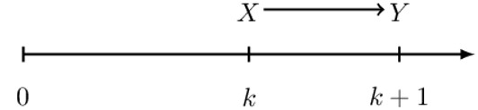
A natural way to depict the time value of money is by timelines. A timeline is some sought of a number line, where at the bottom of the timelines are the units of the time which can be in months, years, quarters (once every three months) or semi-annual (once every six months) or biannual (once every two years) periods, etc. On top of the timeline are money amounts. However, when you are using a particular time unit, be consistent.
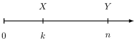
For example, consider a time unit in years and the following timeline.
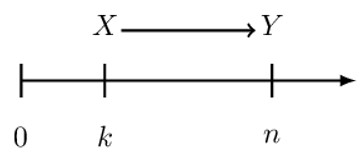
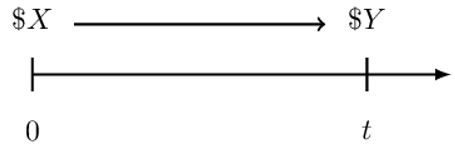
The idea of the time value of money is that over time, you will gain interest on your money. That is, the amount X at time k would have increased to Y at time n. In other words, we would say the amount X at time k is equivalent to Y at time n, assuming that \( \text{Y}>\text{X} \).
The movement of money X at time k to Y at time n is termed as the accumulation of money. In other words, Y is the “accumulated value of X.”
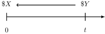
On the other hand, if we move money backward in time, we are “discounting,” and thus, X is called the “discounted value of” Y.
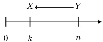
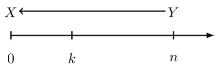
However, if we discount Y to time 0, then X is called the “the present value of” Y.
Now we wish to mathematically relate X and Y now that we know they are not equal. Assume that we know the value of X (at time k), and we wish to determine the value of Y (at time n). To find Y, we multiply X by the periodic accumulation factor (paf), mathematically represented as:
$$ \text{Y}=\text{X}.\text{pa}\text{f}_\text{k}^\text{n} $$
Where
\( \text{pa}\text{f}_\text{k}^\text{n} \) = periodic accumulation factor from time k to time n.
Note that this is not a standard notation, but it is better for the understanding of this material. The notation is analogous to integral calculus, which makes it more palatable.
Now assume that we know Y (at time n), and we wish to calculate X (at time k). We multiply Y by the periodic discount factor from time n back to k. That is,
$$ \text{X}=\text{Y}.\text{pd}\text{f}_\text{n}^\text{k} $$
Where,
\( \text{pd}\text{f}_\text{n}^\text{k} \) = periodic discount factor from time n to time k.
Note that:
$$ \text{pa}\text{f}_\text{k}^\text{n}.\text{pd}\text{f}_\text{n}^\text{k}=1 $$
That is, if you accumulate a unit amount of money and then discount it within the same length of time, then you should get the initial amount you accumulated; otherwise, there is no consistency. Therefore, if
$$ \text{pa}\text{f}_\text{k}^\text{n}.\text{pd}\text{f}_\text{n}^\text{k}=1\Rightarrow \text{pa}\text{f}_\text{k}^\text{n}=\frac{1}{\text{pd}\text{f}_\text{n}^\text{k}} $$
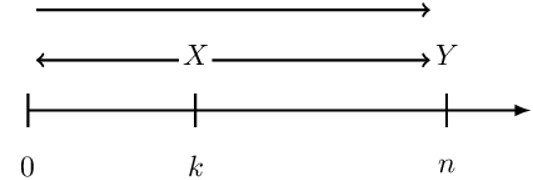
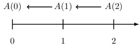
Now consider when in the timeline, there is an intermediate time n as shown below:
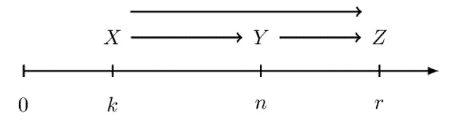
Assume that we want to accumulate from time k to time r. We can do this in two ways: the left- and right-hand sides of the following equation.
$$ \text{pa}\text{f}_\text{k}^\text{r}=\text{pa}\text{f}_\text{k}^\text{n}.\text{pa}\text{f}_\text{n}^\text{r} $$
That is, we can directly accumulate from time k to r or indirectly by first accumulating from time k to time n, then take that amount and accumulating it from time n to time r.
Analogously for the periodic discount factors:
$$ \text{pd}\text{f}_\text{r}^\text{k}=\text{pd}\text{f}_\text{r}^\text{n}.\text{pd}\text{f}_\text{n}^\text{k} $$
At time 0, 100 is deposited into an interest-bearing account. At time 5 the deposit has grown to 240, and at time 7 the deposit has grown to 300.
If an additional 100 was deposited into the account at time 5, how much would have been in the account at time 7?
Consider the following timeline which summarizes the whole question:
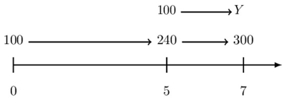
Intuitively, our answer would be 300+Y.
To determine the value of Y, let us focus on the part of the timeline where the 240 at time 5 accumulates to 300 at time 7. Therefore,
$$ 240\cdot \text{pa}\text{f}_5^7=300\Rightarrow \text{pa}\text{f}_5^7=\frac{300}{240}=1.25 $$
We can determine the value of Y because we have determined the value of \(\text{pa}\text{f}_5^7 \). Thus,
$$ \begin{align*} \text{Y}&=100\times\text{pa}\text{f}_5^7=100\times1.25=125 \\ \therefore300+\text{Y}&=300+125=425 \end{align*} $$
At time 0, 100 is deposited into an interest-bearing account. At time 5 the deposit has grown to 240, and at time 7 the deposit has grown to 300.
If an additional amount X was deposited into the account at time 5, then there would have been 1050 in the account at time 7.
Determine X.
Consider the following timeline that summarizes the whole question.
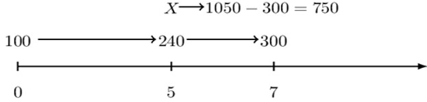
From the timeline, we can see that our answer is
$$ \text{X}=750\cdot{\text{pd}\text{f}}_7^5 $$
Now, focus on the timeline where 240 at time 5 accumulates to 300 at time 7. Then,
$$ 240\cdot \text{pa}\text{f}_5^7=300\Rightarrow \text{pa}\text{f}_5^7=\frac{300}{240}=1.25 $$
Using the relationship,
$$ \text{pd}\text{f}_{\text{n}}^{\text{k}}=\frac{1}{\text{pa}\text{f}_{\text{k}}^{\text{n}}}\Rightarrow \text{pd}\text{f}_{7}^{5}=\frac{1}{1.25}=0.8 $$
And so,
$$ \text{X}=750\cdot \text{pd}\text{f}_7^5=750\cdot0.8=600 $$
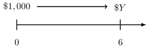
Consider the following timeline:
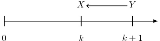
v-notation is a special case when the periodic discount factor over one period is constant. That is, \( \text{pd}\text{f}_{\text{k}+1}^\text{k} \) is a constant. If this is the case, then we just write:
$$ \text{v}=\text{pdf} $$
Therefore, considering the timeline above, we could write:
$$ \text{X}=\text{Y}.\text{v} $$
Where v=pdf in the context that it does not depend on time \( \text{k}+1 \) going back to time k. In other words, if you discount from time 3 back to time 2 or from time 102 back to time 101, the discount factor v will be the same.
Note that we are using the term “periodic” discount factor because we are using a general time unit. So, if our time units were in years, then v will be termed as an “annual” discount factor. That is:
$$ \text{v}=\text{adf} $$
And for months,
$$ \text{v}=\text{mdf} $$
And so on.
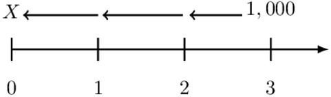
Now assume that we want to discount a Y value for two periods instead of one period using the periodic discount factor v.
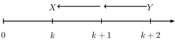
Using the properties studied earlier, then,
$$ \text{X}=\text{Y}.\text{v}.\text{v}=\text{Y}.\text{v}^2 $$
Where
$$ \text{v}=\text{pdf} $$
Note that the power of the discount factor does not necessarily be an integer, it can be a decimal, such as 1.5, depending on the length of the discounting period.
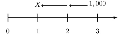
Now consider the equation
$$ \text{X}=\text{Y}.\text{v} $$
We can make Y the subject so that:
$$ \text{Y}=\text{X}.\frac{1}{\text{v}}=\text{X}\text{v}^{-1} $$
The timeline also changes:
In other words,
$$ \text{paf}=\text{v}^{-1} $$
This is intuitive from the fact that,
$$ \text{pa}\text{f}_\text{k}^\text{n}=\frac{1}{\text{pd}\text{f}_\text{n}^\text{k}} $$
Suppose the quarterly discount factor equals 0.98. Determine the equivalent annual accumulation factor.
We are given \( \text{qdf}=0.98 \); furthermore, we seek the equivalent annual accumulation factor (aaf). Then,
$$ \text{qdf}=0.98\Rightarrow\text{qaf}=0.98^{-1} $$
Now intuitively, the annual accumulation factor (aaf) is equivalent to four quarterly accumulation factors:
$$ \text{aaf}=\text{qaf}.\text{qaf}.\text{qaf}.\text{qaf}=\text{qaf}^4 $$
Therefore,
$$ \text{aaf}=\text{qa}\text{f}^4=\left(0.98^{-1}\right)^4=0.98^{-4}=1.0842 $$
An account credits interest in such a way that the monthly accumulation factor is constant, regardless of the month in which the accumulation occurs.
The present value, 2 years before a payment of 4,000, plus the present value, 4 years before the payment of 10,000, sums to 9,801.
Determine the monthly accumulation factor for this account.
Note that the question states that “the monthly accumulation factor is constant, regardless of the month in which the accumulation occurs,” which tells us that we can use the v-notation. For this problem, we can either work in months or years.
Let us work in months. Note that we are starting at time 0, and hence we are dealing with present values. So the timeline for this problem is as shown below:
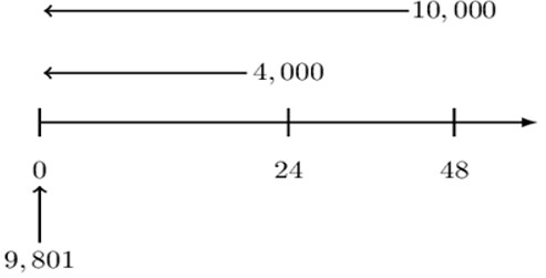
$$ \text{v}=\text{mdf} $$
Intuitively, the equation of value is given by:
$$ 9,801=4,000\text{v}^{24}+10,000 \text v^{48} $$
Now let \( \text{x}=\text{v}^{24} \) then
$$ 9,801=4,000\text{x}+10,000\text{x}^2 $$
We can rewrite the equation as:
$$ 10,000\text{x}^2+4,000\text{x}-9,801=0 $$
Which is a quadratic equation. Using the quadratic formula,
$$ \text{x}=\frac{-\text{b}\pm\sqrt{\text{b}^2-4\text{ac}}}{2\text{a}} $$
Where a=10,000, b=4,000, and c=-9801, we get:
$$ \text{x}=0.81,-1.21\ $$
Ignore the negative value, then x=0.81, and thus
$$ \text{v}^{24}=0.81\Rightarrow\ \text{v}=\left(0.81\right)^\frac{1}{24}=\text{mdf} $$
However, we need a monthly accumulation factor, then we need:
$$ {\text{maf}=\left(\text{mdf}\right)^{-1}=\text{v}}^{-1}=\left(0.81\right)^{-\frac{1}{24}}=1.008818 \text{ Alternatively }, $$
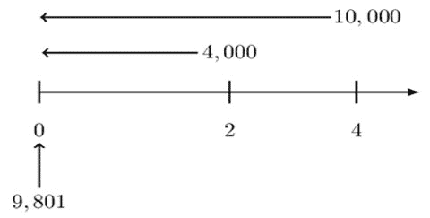
In this case,
$$ \text{v}=\text{adf} $$
Furthermore, the equation of value would be:
$$ 9,801=4,000\text{v}^2+10,000\text{v}^4 $$
Now let \( \text{x}=\text{v}^{24} \) then:
$$ 9,801=4,000\text{x}+10,000\text{x}^2 $$
If we rewrite the equation as:
$$ 10,000{\text{v}}^2+4,000\text{v}-9,801=0 $$
Using the quadratic formula, you get the same result:
$$ \begin{align*} \text{v}&=0.81 \\ \therefore\text{v}^2&=0.81\Rightarrow \text{v}=\text{adf}=0.9 \end{align*} $$
Nevertheless, we need the monthly accumulation factor (maf) so :
$$ \begin{align*} \left(\text{maf}\right)^{12}&=\text{aaf}=\left(\text{adf}\right)^{-1}={0.9}^{-1} \\ \Rightarrow\left(\text{maf}\right)^{12}&={0.9}^{-1}\therefore\ \text{maf}={0.9}^{-\frac{1}{12}}=1.008818 \end{align*} $$
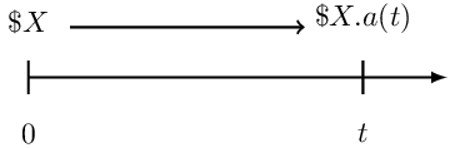
The best way to introduce the accumulation function is by the use of a timeline. Consider the following timeline.
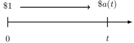
Taking time t as an independent variable, the accumulation function at time t, denoted by a(t), is the accumulated value at time t per dollar invested at time 0. Note that:
$$ \text{a}\left(0\right)=1 \text{ since} $$
Generally, if we have X dollar invested at time 0, we would have \( \text{X}.\text{a}(\text{t}) \) at time t.
This multiplicative property of the accumulation function defines the amount function.
The amount function at time t, denoted by \(\text{A}(\text{t}) \), is the accumulated value at time t when a non-unit amount X is invested at time t=0.
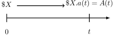
The amount function is defined as:
$$ \text{A}\left(\text{t}\right)=\text{X}.\text{a}(\text{t}) $$
Intuitively, the amount function at time 0 is just X. That is:
$$ \text{A}\left(0\right)=\text{X} $$
This is true by definition since X is the amount of money we have at time 0. Now, consider the equation.
$$ \text{A}\left(\text{t}\right)=\text{X}.\text{a}(\text{t}) $$
We know that \( \text{X}=\text{A}(0) \) so that,
$$ \text{A}\left(\text{t}\right)=\text{A}\left(0\right).\text{a}\left(\text{t}\right)\Rightarrow\ \text{a}\left(\text{t}\right)=\frac{\text{A}\left(\text{t}\right)}{A(0)} $$
This implies that we can recover the accumulation function if we are supplied with the amount functions.
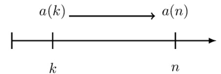
We can link the accumulation functions and the periodic accumulation factors. Consider the following timeline:
We know that:
$$ \begin{align*} \text{Y}&=\text{X}.\text{a}\left(\text{t}\right)=\text{X}.\text{pa}\text{f}_0^\text{t} \\ &\Rightarrow \text{a}\left(\text{t}\right)=\text{pa}\text{f}_0^\text{t} \end{align*} $$
However, you should note that the definition of the accumulation function always starts at time 0.
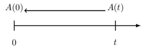
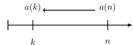
Now assume we want to discount Y back to X:
Intuitively, we will use the periodic discount factor (pdf). Using the definition above:
$$ \text{pdf}_\text{t}^\text{0}=\frac{1}{\text{paf}_0^\text{t}}=\frac{1}{\text{a}(\text{t})} $$
Therefore, the periodic discount factor from time 0 to time t is the reciprocal of the accumulation function. Thus:
$$ \text{X}=\text{Y}.\frac{1}{\text{a}(\text{t})}=\frac{\text{Y}}{\text{a}(\text{t})} $$
A quick way to remember all this is to recognize that to accumulate from time 0 to time t, multiply by \({\text{a}(\text{t})}\) while to discount from time t to time 0, divide by \({\text{a}(\text{t})}\).
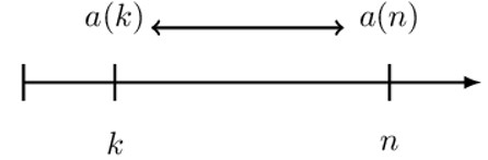
Now consider the general time from the previous discussions:
Then,
$$ \text{Y}=\text{X}.\text{pa}\text{f}_\text{k}^\text{n} $$
However, recall that, by the definition of accumulation function, it must first pass through time 0! Therefore, we need to discount X first to time 0 and then accumulate to time n, as illustrated by the timeline below:
So,
$$ \begin{align*} \text{Y}&=\text{X}\cdot\text{pa}\text{f}_\text{k}^\text{n}=\text{X}\cdot\frac{1}{\text{a}\left(\text{k}\right)}\cdot \text{a}(\text{n}) \\ \Rightarrow \text{pa}\text{f}_\text{k}^\text{n}&=\frac{\text{a}(\text{n})}{\text{a}\left(\text{k}\right)} \end{align*} $$
For the periodic discount factor, we use the fact that:
$$ \begin{align*} \text{pd}\text{f}_\text{n}^\text{k}&=\frac{1}{\text{pa}\text{f}_\text{k}^\text{n}} \\ \Rightarrow\text{pd}\text{f}_\text{n}^\text{k}&=\frac{\text{a}(\text{k})}{\text{a}\left(\text{n}\right)} \end{align*} $$
You are given the following accumulation function values:
$$ \text{a}\left(1\right)=1.2\ \ \ \ \ \ \ \text{a}\left(2\right)=1.5\ \ \ \ \ \ \ \text{a}\left(3\right)=2.0\ \ \ \ \ \ \ \text{a}\left(4\right)=3.0 $$
100 is deposited at time 0, and another 400 is deposited at time 3. Determine the total amount of interest earned between times 2 and 4.
Consider the following timeline, which captures the whole question:
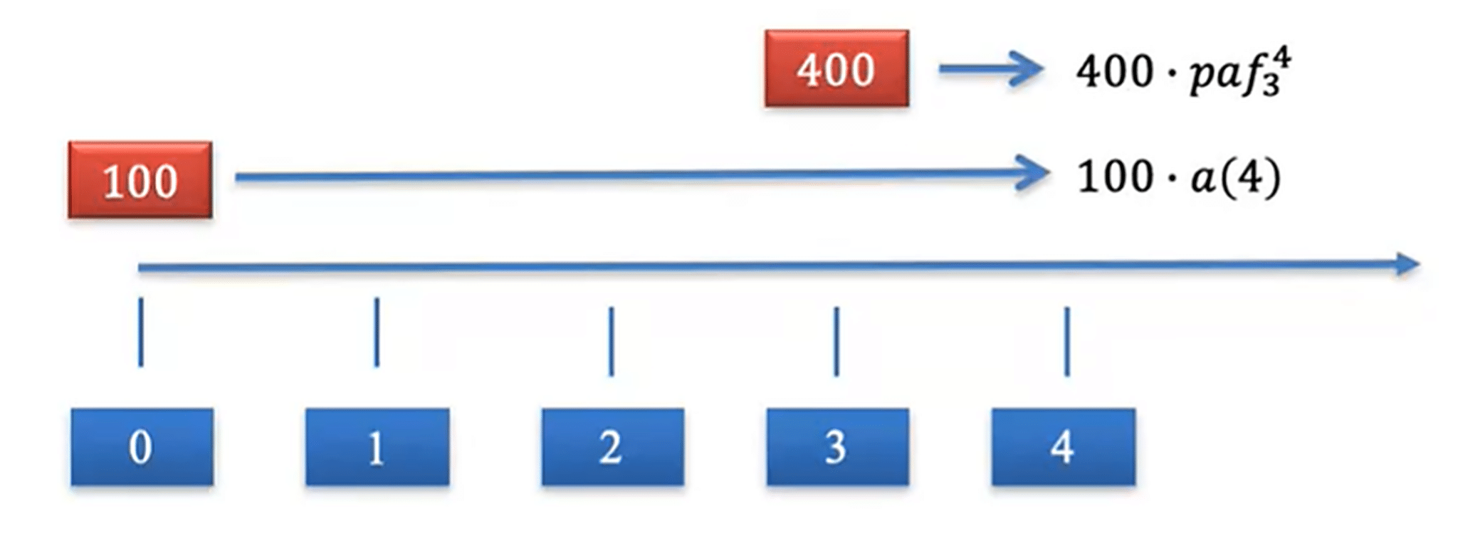 Ideally, the total amount of the interest earned between time 4 and time 2 is essentially the total amount at time 4 less the amount at time 2, less any deposit made between times 2 and 4.
$$ \text{I}[2,4]=\text{A}(4)-\text{A}(2)-(\text{Deposits})[2,4] $$
Where \( (\text{Deposits})[2,4] \) is any deposit made between times 2 and time 4. So,
$$ \begin{align*} \text{I}[2,4]&=\text{A}(4)-\text{A}(2)-400 \\ &=\left[100.\text{a}\left(4\right)+400\text{pa}\text{f}_3^4\right]-\left[100.\text{a}\left(2\right)\right]-400 \\ &=\left[100\times3.0+400\times\frac{\text{a}\left(4\right)}{\text{a}\left(3\right)}\right]-\left[100\times1.5\right]-400\\ &=\left[300+400\times\frac{3.0}{2.0}\right]-550=900-550=350 \end{align*} $$
Alternatively, you can calculate the interest for the 100 deposited at time 0 and the amount of interest for the deposit at time 3 separately, then add them together.
$$ \begin{align*} \text{I}_{\left[2,4\right]}^{\text{d}=100}&=\text{A}_{100}\left(4\right)-\text{A}_{100}\left(2\right)\\ &=100\cdot\text{a}\left(4\right)-100\cdot \text{a}\left(2\right) \\ &=100\cdot3-100\cdot1.5=150 \end{align*} $$
For the 400 deposit,
$$ \text{I}[3,4]\text{d}=400=\text{A}4004-\text{A}400(3) =\text{A}_{400}\left(4\right)-400 $$
Now,
$$ \begin{align*} \text{A}_{400}\left(4\right)&=400\cdot{\text{pa}\text{f}}_3^4=400\cdot\frac{\text{a}\left(4\right)}{\text{a}\left(3\right)}=600 \\ &\Rightarrow\text{I}[3,4]d=400=600-400=200 \end{align*} $$
Therefore the total interest is:
$$ \begin{align*} \text{I}_{\left[2,4\right]}=\text{I}_{\left[2,4\right]}^{\text{d}=100}+\text{I}[3,4]{\text{d}=400}=150+200=350 \end{align*} $$
The simple interest is based on the formula:.
$$ \text{Interest}=\text{principal }\times \text{rate }\times \text{ time} $$
The rate is denoted by i while the time t is always measured in years. The principal is denoted by P and is always the amount at time 0, which is A(0). Consider the 2-year timeline
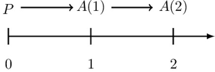
The amount at time 1 is:
$$ \text{A}\left(1\right)=\text{P}+\text{I}_1=\text{P}+\text{P}\cdot\text{i}\cdot1=\text{P}+\text{P}\cdot\text{i}=\text{P}\cdot(1+\text{i}) $$
For the second year, the amount is given by:
$$ \text{A}\left(2\right)=\text{A}\left(1\right)+\text{I}_2=\left(\text{P}+\text{I}_1\right)+\text{I}_2=\left(\text{P}+\text{P}\cdot \text{i}\right)+\text{P}\cdot\text{i}=\text{P}\cdot(1+2\text{i}) $$
Generally, the amount at time t is given by:
$$ \text{A}\left(\text{t}\right)=\text{P}\cdot\left(1+\text{i}.\text{t}\right) $$
Where:
\( \text{A}\left(\text{t}\right)\) – The accumulated amount at time t
\(\text{P}\) – The principal amount
\(\text{t}\) – The number of years
\(\text{i}\) – The rate of interest
Intuitively, the accumulation function under simple interest is given by:
$$ \text{a}\left(\text{t}\right)=1+\text{i}.\text{t} $$
The value of t does not need to be an integer; it can be a fractional value.
The distinguishing feature of this interest is that interest on the principal does not earn further interest
A businessman deposits $1000 in a bank account that pays simple interest of 5% per year. Calculate the accumulated value and hence the simple interest after 3 years.
Solution
$$ \begin{align*} \text{A}\left(\text{t}\right)&=\text{P}\cdot\left(1+\text{i}.\text{t}\right) \\ & =1000(1+0.05 \times 3)=1000(1.15)=$1150 \\ \end{align*} $$
The amount of interest will be given by:
$$ {\textbf{I}}={\textbf{A}}({\textbf{t}})-{\textbf{P}}=1150-1000=$150 $$
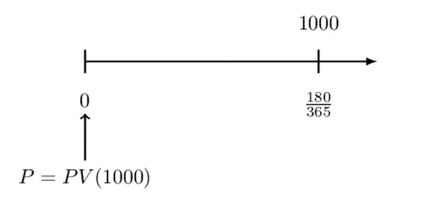
The Government of Canada issues a 180-day Treasury Bill (T-Bill) with a quoted rate of 4% and a redemption value of 1000.
Determine the price of the T-Bill.
Note that with Canadian T-Bills, the quoted rate is a simple interest rate based on a 365-day year.
So the timeline for the above question is as shown below:
 Recall that the accumulation function under simple interest is given by:
$$ \begin{align*} \text{a}\left(\text{t}\right)&=1+.04\text{t} \\ \Rightarrow\text{P}\cdot\text{a}({\frac{180}{365}}) & =1000 \\ \therefore \text{P}\cdot\left(1+0.04\cdot\left({\frac{180}{365}}\right)\right) & =1000\Rightarrow\text{P}=980.66 \end{align*} $$
Unlike simple interest, in compound interest, interest earned earns further interest. That is, the principal is the beginning of the period amount of each period. Consider the following two-period timeline:
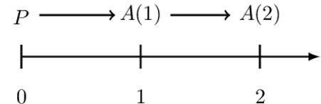
The amount at time 1, A(1) is given by:
$$ \text{A}\left(1\right)=\text{P}+\text{I}_1=\text{P}+\text{P}\cdot\text{i}\cdot1=\text{P}+ \text{P}\cdot\text{i}=\text{P}\cdot(1+\text{i}) $$
For the second period, we have:
$$ \begin{align*} \text{A}\left(2\right)&=\text{A}\left(1\right)+\text{I}_2=\text{A}\left(1\right)+\text{A}\left(1\right)\cdot \text{i}=\text{A}\left(1\right)\cdot\left(1+\text{i}\right) \\ &=\text{P}\cdot(1+\text{i})\cdot\left(1+ \text{i}\right)=\text{P}\cdot{(1+\text{i})}^2 \end{align*} $$
Intuitively, the general formula for an amount at any period t under compound interest is given by:
\(\text{A}(\text{t})=\text{P}\left(1+\text{i}\right)^\text{t}\)
Where:
\(\text{A}\) – The accumulated amount at any time t
\(\text{P}\) – The principal amount
\(\text{t}\) – The number of periods, e.g., years
\(\text{i}\) – The periodic effective rate of interest
From the compound interest formula, it is easy to see that the accumulation function is given by:
$$ \text{a}\left(\text{t}\right)=\left(1+\text{i}\right)^\text{t} $$
A businessman deposits $1000 in a bank account that pays compound interest of 5% per year. Calculate the accumulated value after 3 years.
\( \text{A}(\text{t})=\text{P}\left(1+\text{i}\right)^\text{t} \)
So,
$$ \text{A}(\text{t})=1000\left(1+0.05\right)^3=1000\left(1.05\right)^3=$1157.625 $$
The equation \( \text{A}(\text{t})=\text{P}\left(1+\text{i}\right)^\text{t} \) is called the \(\textbf{ equation of value }\). If we know three of the variables \( \text{A}(\text{t}), \text{P},{\textbf{i}}, \text{ and }{\textbf{t}}, \) we can calculate the remaining unknown variable.
In the case of the simple interest, recall the accumulation is given by:
$$ \text{a}\left(\text{t}\right)=1+\text{i}.\text{t} $$
Also, we know that:
$$ {\text{pa}\text{f}}_\text{k}^{\text{k}+1}=\frac{\text{a}(\text{k}+1)}{\text{a}(\text{k})}=\frac{1+(\text{k}+1)\cdot \text{i}}{1+\text{k}\cdot \text{i}} $$
As seen above, we are not able to cancel out k, and thus we cannot use v-notation since the periodic accumulation function for simple interest depends on k.
However, for the compound interest, the accumulation functions is given by:
$$ \text{a}\left(\text{t}\right)=\left(1+\text{i}\right)^\text{t} $$
And thus,
$$ {\text{pa}\text{f}}_\text{k}^{\text{k}+1}=\frac{\text{a}(\text{k}+1)}{\text{a}(\text{k})}=\frac{{(1+\text{i})}^{\text{k}+1}}{{(1+\text{i})}^\text{k}}=1+\text{i}=\text{paf} $$
Therefore, since the periodic accumulation factor for the compound interest is independent of k, we can use the v-notation. Therefore,
$$ \text{v}={\text{pd}\text{f}}_{\text{k}+1}^\text{k}=\text{pd}\text{f}=\frac{1}{1+\text{i}} $$
Which implies that:
$$ \text{v}^{-1}=1+\text{i}\ \ \ (\text{ the periodic accumulation factor }) $$
This is the amount of money invested now to provide future payments. It is also called discounted value or the current value. It is given by:
$$ PV=F(1+i)^{-n} $$
Where:
\(\text{PV}\) – The present value
\(\text{F}\)- The accumulated value in future
\(\text{i}\) – The rate of interest rate
\(\text{n}\) – The number of years
A company is obliged to pay $10,000 to its investors in five years. The company needs to invest the same money to provide the payment at the stipulated time. What will be the initial amount of this investment at 10% per year compounded interest?
$$ \begin{align*} PV & =F(1+i)^{-n} \\ & =10000(1+0.1)^{-5}=10000(1.1)^{-5}=$6209.21 \\ \end{align*} $$
Put simply, the present value is the amount of money required to be invested now to give a future value \(F\). We define a function \(v=\cfrac {1}{1+i}=(1+i)^{-1}\) and for \(n \ge 1,v^n=(1+i)^{-n}\). It follows immediately that \(\text{PV}=\text{Fv}^{\text n}\).
Therefore, in the example above,
$$ PV=Fv^n, $$
So that in the question \(n=5\) and \(i=0.1\)
$$ \Rightarrow PV=10000(1.1)^{-5}=$6209.21 $$
The values of \(v\) can be directly found from actuarial tables at specified rates of interest.
Note, however, that the net present value is the difference between the present value of the cash inflows and cash outflows. Denoted as NPV, it is mostly used in project appraisal.
Consider a series of payments. The present value of these cash flows is equal to the sum of individual present values. Now, consider payments of \(C_k\) at time \(k=1,2,\dots,n-1,n\) at an effective rate of interest \(i\) corresponding to discount factor \(v\), then the present value of the cash flow is given by:
$$ PV=\sum _{ k=0 }^{ n }{ { C }_{ k }{ v }^{ k } } \dots \dots \dots \dots \dots (1) $$
The future value of these streams of payment is given by:
$$ FV={ \left( 1+i \right) }^{ n }\left( PV \right) ={ \left( 1+i \right) }^{ n }\left( \sum _{ k=0 }^{ n }{ { C }_{ k }{ v }^{ k } } \right) =\sum _{ k=0 }^{ n }{ { C }_{ k }{ \left( 1+i \right) }^{ n-k } } \dots \dots \dots \dots \left( 2 \right) $$
Equations (1) and (2) are called equations of value because each can be used to find the missing variables.
Recall that for the simple interest:
$$ \text{Interest}=\text{Principal } \times \text{Rate } \times \text{Time} $$
We use the same analogy in the case of the simple discount. However, simple interest is paid at the end of the period, based on the amount of money (i.e., principal) at the beginning of the period. On the other hand, the discount is paid at the beginning of the period, based on the amount of money (i.e., principal) at the end of the period.
Consider the following timeline:
Now let d be the simple discount rate of interest so that the amount of discount is given by:
$$ \text{D}=\text{A}\left(\text{t}\right).\text{d}.\text{t} $$
(Note that for simple discount, the principle is at the end of the period, \( \text{A}\left(\text{t}\right)=\text{P}): \)
Now since the discount is paid at the beginning of the period then,
$$ \text{A}\left(0\right)=\text{A}\left(\text{t}\right)-\text{D} $$
If we substitute the value for D in the equation above, we get:
$$ \text{A}\left(0\right)=\text{A}\left(\text{t}\right)-\text{D}=\text{A}\left(\text{t}\right)-\text{A}\left(\text{t}\right).\text{d}.\text{t} =\text{A}(\text{t})(1-\text{d}.\text{t}) $$
For the accumulation function, we know that:
$$ \text{A}\left(0\right)=\text{A}\left(\text{t}\right)\left(1-\text{d}.\text{t}\right)\Rightarrow\frac{\text{A}\left(0\right)}{\text{A}\left(\text{t}\right)}=\left(1-\text{d}.\text{t}\right) $$
But,
$$ \text{a}\left(\text{t}\right)=\frac{\text{A}\left(\text{t}\right)}{\text{A}\left(0\right)} $$
Therefore,
$$ \text{a}\left(\text{t}\right)=\left(1-\text{d}.\text{t}\right)^{-1} $$
In summary, the simple discount value is given by:
$$ \text{A}\left(0\right)=\text{P}\left(1-\text{d}.\text{t}\right) $$
Where:
\(\text{P}\) – The amount due in the future (Principal)
\(\text{t}\) – The number of years
\(\text{d}\) – The rate of simple discount
What is the discounted value of $10,000 at a simple discount rate of 5% per year for 3 years?
$$ \text{A}\left(0\right)=\text{P}\left(1-\text{d}.\text{t}\right)=10000\left(1-3\times0.05\right)=10000\left(0.85\right)=$8,500 $$
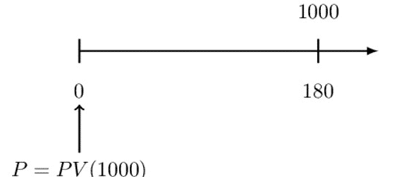
The US Government issues a 180-day Treasury Bill (T-Bill) with a quoted rate of 4% and a redemption value of 1000.
Determine the price of the T-Bill.
While with Canadian T-Bills, the quoted rate is a simple interest rate based on a 365-day year. With US T-Bills, the quoted rate is a simple discount rate based on a 360-day year.
Consider the following timeline:
From the question,
$$ \text{d}=0.04\ (\text{ simple })\Rightarrow\ \ \text{a}(\text{t})=\left(1-.04\text{t}\right)^{-1} $$
Therefore,
$$ \begin{align*} \text{P}\cdot\text{a}\left({\frac{180}{360}}\right)&=1000\Rightarrow \text{P}\cdot\left(1-.04\cdot\left({\frac{180}{360}}\right)\right)^{-1}=1000 \\ &\therefore\therefore\text{P}=980.00 \end{align*} $$
As with compound interest, interest earned earns interest itself. It represents the amount to be invested now to accumulate to amount \(C\) in the future. Consider the following timeline:
Let,
\( \text{d} = \text{ periodic effective discount rate (periodic edr) } \)
Using the analogy of discount rate (the interest is paid at the beginning of the period, and the principal is the amount at the end of the period):
$$ \text{A}\left(1\right)=\text{A}\left(2\right)-\text{D}_2 $$
But,
$$ \text{D}_2=\text{A}\left(2\right).\text{d} $$
So,
$$ \begin{align*} \text{A}\left(1\right)&=\text{A}\left(2\right)-\text{A}\left(2\right).\text{d}=\text{A}\left(2\right).(1-\text{d}) \\ &\therefore \text{A}\left(1\right)=\text{A}\left(2\right).(1-\text{d}) \end{align*} $$
Similarly,
$$ \begin{align*} \text{A}\left(0\right)&=\text{A}\left(1\right)-\text{D}_1 \\ & =\text{A}\left(2\right).\left(1-\text{d}\right)-\text{d}.(\text{A}\left(2\right).(1-\text{d})) \\ &=\text{A}\left(2\right)\left[\left(1-\text{d})-\text{d}\left(1-\text{d}\right)\right)\right]\\ \Rightarrow\text{A}\left(0\right)&=\text{A}\left(2\right)\left(1-\text{d}\right)^2 \end{align*} $$
So generally,
$$ \text{A}\left(0\right)=\text{A}\left(\text{t}\right)\left(1-\text{d}\right)^\text{t} $$
Which can be written as:
$$ \frac{\text{A}\left(0\right)}{\text{A}\left(\text{t}\right)}=\left(1-\text{d}\right)^\text{t} $$
But
$$ \begin{align*} \text{a}\left(\text{t}\right)&=\frac{\text{A}\left(\text{t}\right)}{\text{A}\left(0\right)}\\ &\Rightarrow\text{a}\left(\text{t}\right)^{-1}=\left(1-\text{d}\right)^\text{t} \\ &\therefore\text{a}\left(\text{t}\right)=\left(1-\text{d}\right)^{-\text{t}} \end{align*} $$
The relationship between the v-notation and the effective discount rate is given by:
$$ \text{v}=1-\text{d} $$
What is the discounted value of $10,000 at the compound discount rate of 5% per year for 3 years?
We know that:
$$ \text{A}\left(0\right)=\text{A}\left(\text{t}\right)\left(1-\text{d}\right)^\text{t}=10,000\left(1-0.05\right)^3=$\ 8,573.75 $$
Nominal rates, on the other hand, are those rates that are paid more than once per unit time period. On the other hand, effective rates are compound rates where interest is paid once per unit time. It is referred to as an effective rate of interest if it is paid at the end of the period and an effective discount rate if it is paid at the beginning of the period.
It is denoted by \(i^{(m)}\). It is also referred to as convertible m-thly or compounded m-thly. It is defined to be an interest of \(\cfrac {i^{(m)}}{m}\) applied to each m-th of a time period.
For instance, \(i^{(12)}\) refers to nominal rates convertible monthly while \(i^{(4)}\) refers to a nominal rate of interest convertible quarterly. In other words \(i^{(m)}\) is equivalent to \(\cfrac {i^{(m)}}{m}\) monthly effective rate of interest. For example, the monthly effective interest of 2% equals \(12 \times 2\%=24\%\) interest rate compounded monthly. So, \(i^{(12)}=24\%.\) The accumulation factor under the nominal rate of interest is given by \(\left(1+\cfrac {i^{(m)}}{m}\right)^m\)
Using the equivalent rates principle, the relationship between the nominal interest and effective rates is given by:
$$ 1+i=\left(1+\cfrac {i^{(m)}}{m}\right)^m $$
Note that \(i^{(1)}=i\), which confirms the definition of effective rate of interest.
Rearranging the above equation, we get:
$$ i^{(m)}=m \left[(1+i)^{\frac {1}{m}}-1 \right] $$
This equation is used to convert between effective and nominal rates of interest as quickly as you can.
Convert 6% per year effective to nominal rate convertible quarterly.
$$ \begin{align*} i^{(m)} &= m\left[(1+i)^{\frac {1}{m}}-1 \right] \\ i^{(4)} &=4\left[(1+0.06)^{\frac {1}{4}}-1 \right]=4 \left[(1.06)^{\frac {1}{4}}-1 \right]=0.058695=5.8695\% \\ \end{align*} $$
The nominal rate is the multiple of the effective rates of interest and we cannot use it directly to accumulate and discount. Hence, it is advisable to convert to nominal interest rate to effective interest rates and use the accumulation and discounting formula as before:
$$ \begin{align*} a(n) & =(1+i)^n \\ v(n) & =v^n=(1+i)^{-n} \\ \end{align*} $$
$5000 is deposited in a bank account that pays 8% nominal interest rate per annum convertible semi-annually. Find the accumulated value after 3 years.
We are given that \(i^{(2)}=8\%.\) We know that:
$$ 1+i=\left(1+ \cfrac {i^{(m)}}{m}\right)^m \Rightarrow i=\left(1+ \cfrac {i^{(m)}}{m} \right)^m-1=\left(1+\cfrac {i^{(2)}}{2} \right)^2-1 =0.0816=8.16\% $$
Now,
$$ A(n)=(1+i)^n=5000(1.0816)^3=$6326.60 $$
Application of nominal rate of interest can be done directly by converting the unit of time as per the frequency with which the nominal rate is convertible and use \(\cfrac {i^{(m)}}{i}\) as the effective rate of interest per unit time. For instance, we can calculate the above example as follows:
\(i^{(2)}=8\%\) is equivalent to \(\cfrac {8\%}{2}=4\%\) half-yearly effective rate of interest and 3 years is equivalent to \({\cfrac {3}{0.5}}=6\) half-years. The accumulation will be:
\(5000(1.04)^6=$6326.60\)
$$ 5,000\left(1+\frac{8\%}{2}\right)^{3\times2}=5000\left(1.04\right)^6=$6,326.60 $$
Which gives the same answer as above.
Bob deposits 1,000 into an account, which credits interest using an interest rate of 8% compounded quarterly. How much will Bob have after 6 months?
We are given: \( \text{i}^{\left(4\right)}=0.08 \) so that, \( qeir=\frac{0.08}{4}=0.02 \)
$$ \text{A}\left(6\right)=1,000.\text{a}\left(6\right)=1000\left(1+\text{i}\right)^{\frac{6}{12}\times4}=1000\left(1+0.02\right)^2=1,040.40 $$
Amy deposits 1000 into an account, which credits interest using a quarterly effective interest rate of 2%. How much will Amy have in the account after 6 months?
The typical timeline for this problem is as shown below:
Therefore,
$$ \text{Y}=1000.\text{a}\left(6\right)=1000\left(1+\text{i}\right)^{\frac{6}{12}\times4}=1000\left(1+0.02\right)^2=1,040.40 $$
Note that we are given a “quarterly effective interest rate of 2%,” so we use it directly! Moreover, we need to convert the “ 6 months” into quarters, which are essentially 2 quarters.
It is denoted by \(d^{(m)}\) and described as the rate of discount convertible m-thly or compounded m-thly. For instance, \(d^{(12)}\) is referred to as the nominal rate of interest convertible monthly and \(d^{(4)}\) is the nominal rate of interest convertible quarterly.
It is the rate of discount of \(\cfrac {d^{(m)}}{m}\) applied to each m-th period.
Using a similar argument as the compound rate of interest, the relationship between effective and nominal rate of interest can be obtained using the equivalence principle as follows:
$$ 1-d= \left(1-\cfrac {d^{(m)}}{m }\right)^m $$
Rearranging (making \(\text d^{(\text m)})\) the subject of the formula), we get:
$$ d^{(m)}=m\left[1-(1-d)^{\frac {1}{m}} \right] $$
Convert 5% per year effective discount rate of interest as a nominal rate convertible monthly.
We know that:
$$ \begin{align*} d^{(m)} & =m \left[1-(1-d)^{\frac {1}{m}} \right] \\ \Rightarrow d^{(12)} & =12 \left[1-(1-0.05)^{\frac {1}{12}} \right]=0.05118=5.118\% \\ \end{align*} $$
Instead of using a nominal rate of discount, it is usually more convenient to convert the nominal discount rate of interest to an effective rate of interest or the other way round. This can be done as follows:
We know that \(v=1-d\).
$$ \begin{align*} \Rightarrow d^{(m)} & =m\left[1-(v)^{\frac {1}{m}} \right] \\ & =m \left[1-(1+i)^{-\frac {1}{m}} \right] \\ \end{align*} $$
Make \(1+i\) the subject of the formula. To give:
$$ 1+i=\left(1-\cfrac {d^{(m)} }{m} \right)^{-m} $$
Calculate the annual effective of interest equivalent to a discount rate of 8% convertible quarterly.
We are given that:
$$ d^{(4)}=0.08 $$
And we know that,
$$ 1+i=\left( 1-\cfrac { d^{ (m) } }{ m } \right) ^{ -m }\Rightarrow i=\left( 1-\cfrac { d^{ (m) } }{ m } \right) ^{ -m }-1 $$
So,
$$ i=\left(1-\cfrac {d^{(m)} }{m} \right)^{-m}-1=\left(1-\cfrac {0.08}{4} \right)^{-4}-1=0.084166=8.4166\% \quad per \quad year $$
An account credits interest using a 9% interest rate compounded monthly for the first year, and an 8% discount rate compounded quarterly for the second year. Determine the accumulated value after two years of a deposit of 1000.
First year: \(\text{i}^{({12})}={{0}}.{{09}}\)
Second year: \( \text{d}^{(\text{4})}={{0}}.{{08}}\)
So the accumulated value after two years is given by:
$$ \text{A}\left(2\right)=1,000\left(1+\frac{{0}.{09}}{12}\right)^{1\times 12}\left(1-\frac{{0}.{08}}{4}\right)^{-1\times 4}=1,185.87 $$
The nominal rate of discount is a multiple of the effective discount rate for a given unit of time, so we cannot use it directly to accumulate or discount. So the formulas above, we convert the nominal discount rate to effective rates, which we can use.
Note that:
$$ \begin{align*} v(n) & =(1-d)^n \quad And \\ a(n) & =\cfrac {1}{v(n)} =(1-d)^{-n} \\ \end{align*} $$
Another method is to convert the nominal discount rate of interest to effective interest rates and use the following formulas, as stated previously.
$$ \begin{align*} a(n) & =(1+i)^n \\ v(n) & =v^n=(1+i)^{-n} \\ \end{align*} $$
$5000 is deposited in a bank account that pays 8% nominal discount rate per annum convertible semi-annually. Find the accumulated value after 3 years.
We are given the \(d^{(2)}=0.08\)
We know that:
$$ i=\left(1- \cfrac {d^{(m)} }{m} \right)^{-m}-1. $$
So,
$$ i=\left(1-\cfrac {0.08}{2} \right)^{-2}-1=0.085069=8.5069\% $$
Now,
$$ \begin{align*} a(t) & =(1+i)^t \\ \Rightarrow A(3) & =5000(1.085069)^3=$6387.66413 \\ \end{align*} $$
The force of interest is the nominal rate of interest compounded continuously. It is also called the continuously compounded rate. It is denoted by \(\delta\) and defined as:
$$ \lim _{ m\rightarrow \infty }{ { i }^{ \left( m \right) }=\delta } $$
The relationship between the effective rate of interest and force of interest can be derived as follows (briefly):
We know that by the principle of equivalent rates of interest,
$$ 1+i=\left(1+\cfrac {i^{(m)} }{m} \right)^m $$
Taking limit \({ m\rightarrow \infty }\) on the right-hand side of this equation we have:
$$ 1+i=\lim _{ m\rightarrow \infty }{ { \left( 1+\cfrac { i^{ (m) } }{ m } \right) ^{ m } }={ e }^{ { i }^{ \left( \infty \right) } }={ e }^{ \delta } } $$
In this case, it is a case called a constant force of interest.
Note that Euler’s rule was used here. That is:
$$ \lim _{ m\rightarrow \infty }{ { \left( 1+\cfrac { x }{ m } \right) ^{ m } }={ e }^{ { x } } } $$
So,
$$ 1+i=e^{\delta}\Rightarrow \delta =ln(1+i) $$
The force interest is a yearly rate, so we can easily convert it to an effective rate of interest using the relationship obtained above:
$$ 1+i=e^{\delta}\Rightarrow \delta=ln(1+i) $$
$5000 is deposited in a bank account that pays 8% force of interest per annum convertible semi-annually.
Find the accumulated value after 3 years.
We are given that \(\delta=0.08\) but we now that \(1+i=e^{\delta}. \)
$$ i=e^{\delta}-1=e^{0.08}-1=0.0832871=8.3287\%. $$
So,
$$ \therefore A(0,3)=5000(1.0832871)^3=$6356.2457 $$
It is interesting, however, to note that we can obtain accumulation value without conversion. First, consider the following explanation:
We know that the accumulation function for compound interest is:
$$ \text{a}\left(\text{t}\right)=\left(1+\text{i}\right)^\text{t} $$
But,
$$ {{1}}+\text{i}=\textbf{e}^{\delta} $$
If we plug in the accumulation factor, then:
$$ \text{a}\left(\text{t}\right)=\left(\text{e}^\delta\right)^\text{t}=\text{e}^{\text{t}\delta} $$
Therefore, the above example could have been calculated as:
$$ \text{A}\left(3\right)=5000\times\text{e}^{3\times0.08}=$6,356.2457 $$
Note that we can use the v-notation when it comes to the constant force of interest. Recall that:
$$ \begin{align*} \text{a}\left(\text{t}\right)&=\left(\text{e}^\delta\right)^\text{t}=\text{e}^{\text{t}\delta} \\ \text{aa}\text{f}_\text{k}^{\text{k}+1\ }&=\frac{\text{a}\left(\text{k}+1\right)}{\text{a}(\text{k})}=\frac{\text{e}^{\delta\left(\text{k}+1\right)}}{\text{e}^{\delta \text{k}}}=\frac{\text{e}^{\delta \text{k}}.\text{e}^\delta}{\text{e}^{\delta \text{k}}}=\text{e}^\delta=\text{aaf} \end{align*} $$
Therefore, since it is independent of time k, we can use the v-notation. Thus given:
$$ \text{a}\left(\text{t}\right)=\text{e}^{\text{t}\delta} $$
Where t is measured in years and \( {\delta} \) is a constant force of interest,
$$ \text{adf}=\text{e}^{-\text{t}\delta}\Rightarrow\ \text{aaf}=\text{v}^{-1}=\text{e}^\delta $$
An account credits interest using a 6% rate compounded bi-annually for the first year, a 6% discount rate compounded annually for the second year, and a force of interest of 6% for the third year.
How much must be invested in order to have 1,000 at the end of three years?
Consider the following the following timeline:
We can use v-notation to make work easier. So the equation of value is:
$$ \text{X}=1000.\text{v}_1.\text{v}_2.\text{v}_3 $$
For the third year:
$$ \text{v}_3=\text{e}^{-0.06} $$
For the second year:
$$ \text{v}_2=\left(1-\text{d}\right)^1=1-0.06=0.94 $$
For the first year:
$$ \text{v}_1=\left(1+\frac{0.06}{\frac{1}{2}}\right)^{-1\times\frac{1}{2}} $$
So,
$$ \text{X}=1000\times.\text{e}^{-0.06}.\times0.94.\left(1+\frac{0.06}{\frac{1}{2}}\right)^{-1\times\frac{1}{2}}=836.49 $$
The previous discussion has been about the constant force of interest. As a function of time, the force of interest can be defined as the instantaneous change in the value of the fund, expressed as the percentage of the current fund value.
Mathematically, we can define force interest as:
$$ \delta_\text{t}=\frac{\text{a’}(\text{t})}{\text{a}(\text{t})} $$
Where t is measured in years.
For instance, recall that for simple interest, the accumulation function is given as:
$$ \text{a}\left(\text{t}\right)=1+\text{i}.\text{t} $$
So that,
$$ \delta_\text{t}=\frac{\text{a’}(\text{t})}{\text{a}(\text{t})} =\frac{\left[1+\text{i}\cdot\text{t}\right]^{‘}}{1+\text{i}\cdot\text{t}}=\frac{\text{i}}{1+\text{i}\cdot\text{t}} $$
Also, for the simple discount rate, the accumulating function is given by:
$$ \text{a}\left(\text{t}\right)=\left(1-\text{d}\cdot \text{t}\right)^{-1} $$
Then,
$$ \delta_\text{t}=\frac{\text{a}^\prime(\text{t})}{\text{a}\left(\text{t}\right)}=\frac{\left[\left(1-\text{d}\cdot \text{t}\right)^{-1}\right]^\prime}{\left(1-\text{d}\cdot \text{t}\right)^{-1}}=\frac{{-\left(1-\text{d}\cdot \text{t}\right)}^{-2}(-\text{d})}{\left(1-\text{d}\cdot \text{t}\right)^{-1}}=\frac{\text{d}}{1-\text{d}\cdot \text{t}} $$
The accumulation function can be given in a different form, such as:
$$ \text{a}\left(\text{t}\right)=\text{b}^\text{t} $$
So that,
$$ \delta_\text{t}=\frac{\text{a}^\prime(\text{t})}{\text{a}\left(\text{t}\right)}=\frac{\left[\text{b}^\text{t}\right]^\prime}{\text{b}^\text{t}}=\frac{\text{b}^\text{t}\text{ln}(\text{b})}{\text{b}^\text{t}}=\text{ln}(\text{b}) $$
From the last example, we can see that given an exponential accumulation function, then the force of interest is just the natural log of the base. For instance, let
\( \text{a}\left(\text{t}\right)=\text{e}^{\text{rt}}, \text{ then } \)
$$ \delta_\text{t}=\text{ln}\left(\text{e}^\text{r}\right)=\text{r}=\delta $$
Note that r is a constant so that we can replace it with the \( \delta \).
Account A credits interest using a 10% simple discount rate. Account B uses an interest rate i, compounded semi-annually. At the end of two years, the forces of interest for accounts A and B are equal.
Determine i.
For account A, the accumulation function is given by:
$$ \text{a}\left(\text{t}\right)=\left(1-\text{d}.\text{t}\right)^{-1} $$
This is a simple discount rate, and as shown above, the force of interest is given by:
$$ {\delta}_\text{t}^\text{A}=\frac{\text{d}}{1-\text{d}\cdot \text{t}}=\frac{\text{d}}{1-0.1\text{t}} $$
And after two years with a discount rate of 10%,
$$ {\delta}_{{2}}^\text{A}=\frac{\text{d}}{1-0.1\text{d}\cdot {\text t}}=\frac{0.10}{1-0.10\times 2}=0.125\ $$
For account B,
Since Account B uses an interest rate i, compounded semi-annually, we are, therefore, looking for a semi-annual rate and we can denote that as \(i^2\).
$$ \text{a}\left(\text{t}\right)=\left(1+\frac{\text{i}^{\left(2\right)}}{2}\right)^{2\text{t}} $$
Since the accumulation function is an exponential in the form of \( \text{b}^\text{t} \), then the force of interest is given by:
$$ {\delta}_\text{t}^\text{B}={\text{ln}}\left(1+\frac{\text{i}^{\left(2\right)}}{2}\right)^2 $$
We know that after two years, the forces of interest in accounts A and B will be equal. So,
$$ {\text{ln}}\left(1+\frac{\text{i}^{\left(2\right)}}{2}\right)^2=0.125\ $$
Exponentiating both sides, we get:
$$ \begin{align*} & \Rightarrow\left(1+\frac{\text{i}^{\left(2\right)}}{2}\right)^2 =\text{e}^{0.125} \\ & \therefore \text{i}^{\left(2\right)}=2\left[\text{e}^\frac{0.125}{2}-1\right]=12.9\% \end{align*} $$
From the elementary calculus, we know that \( \frac{\text{d}}{\text{dx}}\text{ln}{\left(\text{f}\left(\text{x}\right)\right)}=\frac{\text{f}^\prime\left(\text{x}\right)}{\text{f}\left(\text{x}\right)}. \text{ Therefore}, \)
$$ \delta_\text{t}=\frac{\text{a}^\prime\left(\text{t}\right)}{\text{a}\left(\text{t}\right)}=\frac{\text{d}}{\text{dt}}\text{ln}{\left(\text{a}\left(\text{t}\right)\right)} $$
Integrating both sides, we get (let c be a constant):
$$ \begin{align*} \int_{\text{c}}^{\text{t}}{\delta_\text{t}\text{dt}}&=\int_{\text{c}}^{{\text{t}}}{{\frac{\text{d}}{\text{dt}}\text{ln}{\left(\text{a}\left(\text{t}\right)\right)}}} \\ \Rightarrow \text{ln}{\left(\text{a}\left(\text{t}\right)\right)}&=\int_{\text{c}}^{\text{t}}{\delta_\text{t}\text{dt}} \end{align*} $$
Now let t=0, then
$$ \text{ln}{\left(\text{a}\left(0\right)\right)}=\int_{\text{c}}^{0}{\delta_\text{t}\text{dr}} $$
But we also know that,
$$ \text{a}\left(0\right)=1 $$
So that,
$$ \begin{align*} \text{ln}{\left(1\right)}&=\int_{\text{c}}^{0}{\delta_\text{t}\text{dt} } \\ 0&=\int_{\text{c}}^{0}{\delta_\text{t}\text{dt}}\\ &\therefore \text{c}=0 \end{align*} $$
Thus,
$$ \text{ln}{\left(\text{a}\left(\text{t}\right)\right)}=\int_{0}^{\text{t}}{\delta_{\text{r}}\text{dr}} $$
And if we solve for \( \text{a}\left(\text{t}\right) \) we get,
$$ \text{a}\left(\text{t}\right)=\text{e}^{\int_{0}^{\text{t}}{\delta_{\text{r}}\text{dr}}} $$
Sometimes the expression above is written as:
$$ \text{a}\left(\text{t}\right)=\exp{\left(\int_{0}^{\text{t}}{\delta_{\text{r}}\text{dr}}\right)} $$
To find the present value (discounting), we use the following principle. We know that:
$$ \begin{align*} \text{pa}\text{f}_\text{k}^\text{n}&=\frac{\text{a}(\text{n})}{\text{a}(\text{k})}=\frac{\text{e}^{\int_{0}^{\text{n}}{\delta_\text{t}\text{dt}}}}{\text{e}^{\int_{0}^{\text{kn}}{\delta_\text{t}\text{dt}}}}=\text{e}^{\text{e}^{\int_{0}^{\text{n}}{\delta_\text{t}\text{dt}-\int_{0}^{\text{k}}{\delta_\text{t}\text{dt}}}}}=\text{e}^{\int_{\text{k}}^{\text{n}}{\delta_\text{t}\text{dt}}} \\ &\therefore\text{pa}\text{f}_\text{k}^\text{n}=\text{e}^{\int_{\text{k}}^{\text{n}}{\delta_\text{t}\text{dt}}} \end{align*} $$
Using the same process, the periodic accumulation factor is
$$ \text{pd}\text{f}_{\text{n}}^{\text{k}}=\text{v}=\text{e}^{\int_{\text{n}}^{\text{k}}{\delta_\text{t}\text{dt}}}=\text{e}^{-\int_{\text{k}}^{\text{n}}{\delta_\text{t}\text{dt}}} $$
The force of interest is given to be \( \delta\left(\text{t}\right)=0.02+0.01t. \).
Calculate the accumulated value of $5000 invested at time 0 for a period of eight years.
We need,
$$ \text{A}\left(8\right)=\text{A}\left(0\right).\text{a}(8) $$
But we know that,
$$ \begin{align*} \text{a}\left(\text{t}\right)&=\text{e}^{\int_{0}^{\text{t}}{\delta_\text{t}\text{dt}}} \\ \text{A}(8)&=5000{.\text{e}}^{\int_{0}^{8}\left(0.02+0.01\text{t}\right)\text{dt}} \\ &=5000\text{e}^{\left[0.02\text{t}+0.005\text{t}^2\right]\begin{matrix}8\\0\\\end{matrix}} \\ &=5000\text{e}^{0.48}=$8,080.3720 \end{align*} $$
The force of interest is given as below:
\( \delta\left(\text{t}\right)=0.13-0.01\text{t} \)
Calculate the present value of $6000 to be received in 6 years.
We need,
$$ 6000\text{pd}\text{f}_{6}^{0} $$
\( \text{v}=\text{pd}\text{f}_\text{n}^\text{k}=\text{e}^{-\int_{\text{k}}^{\text{n}}\delta\left(\text{t}\right)\text{dt}}\Rightarrow6000.\text{v}=6000\text{e}^{-\int_{0}^{6}{0.13-0.01\text{t}\text{dt}}} \\ =6000\text{e}^{-\left[0.13\text{t}-0.005\text{t}^2\right]\begin{matrix}6\\0\\\end{matrix}}=6000\text{e}^{-0.6}=$3,292.87\)
There are exceptional cases of force interest that often appear in actuarial exams. Thus, there are special formulas that are worth memorizing. Now we know that:
$$ \text{a}\left(\text{t}\right)=\text{e}^{\int_{0}^{\text{t}}{\delta_\text{t}\text{dt}}} $$
Given the force of interest \( \delta_\text{t} \) can be written in the form of:
$$ \delta_\text{t}=\text{c}.\frac{\text{f}^\prime(\text{t})}{\text{f}(\text{t})} $$
Where c is a constant and \( \text{f}(\text{t}) \) is the denominator of the force of interest and \( \text{f}^\prime(\text{t}) \) is its derivative, then:
$$ \begin{align*} \int_{0}^{\text{t}}{\delta_\text{t}\text{dt}}&=\int_{0}^{\text{t}}{\text{c}.\frac{\text{f}^\prime(\text{t})}{\text{f}(\text{t})}\text{dt}=\text{c}.\text{ln}{(\text{f}(\text{t}))}}|_0^\text{t} \\ &=\text{c}.[\text{ln}(\text{f}\left(\text{t}\right)-\text{ln}{(\text{f}(0))})] \\ &=\text{c}.\text{ln}{\left(\frac{\text{f}\left(\text{t}\right)}{\text{f}\left(0\right)}\right)} \\ \Rightarrow\ \text{e}^{\int_{0}^{\text{t}}{\delta_\text{t}\text{dt}}} & =\left(\frac{\text{f}\left(\text{t}\right)}{\text{f}\left(0\right)}\right)^\text{c} \end{align*} $$
But,
$$ \begin{align*} \text{a}\left(\text{t}\right)&=\text{e}^{\int_{0}^{\text{t}}{\delta_\text{t}\text{dt}}} \\ \therefore \text{a}\left(\text{t}\right) & =\left(\frac{\text{f}\left(\text{t}\right)}{\text{f}\left(0\right)}\right)^\text{c} \end{align*} $$
To summarize all of the above if the given force of interest can be written in the form of:
$$ \delta_\text{t}=\text{c}.\frac{\text{f}^\prime(\text{t})}{\text{f}(\text{t})} $$
Then,
$$ \text{a}\left(\text{t}\right)=\left(\frac{\text{f}\left(\text{t}\right)}{\text{f}\left(0\right)}\right)^\text{c} $$
An amount X is deposited into an account on January 1, 2015. The value of the deposit on January 1, 2019, is 1,000. The account credits interest using a force of interest \( \delta_\text{t}=\frac{\text{t}}{\text{t}^2+9} \) where t is the number of years after January 1, 2015.
Determine X.
Let
January 1, 2015, corresponds to t=0.
January 1, 2019, corresponds to t=4.
We are trying to find the value of 1,000 at time 0 so that the equation of value is given by:
$$ \text{X}=1000.\text{pd}\text{f}_4^0=1000.\frac{\text{a}(0)}{\text{a}(4)} $$
Given,
$$ \delta_\text{t}=\frac{\text{t}}{\text{t}^2+9} $$
Then,
$$ \text{f}\left(\text{t}\right)=\text{t}^2+9 $$
Which implies that:
$$ \text{f}^\prime\left(\text{t}\right)=2\text{t} $$
Therefore, we can write:
$$ \begin{align*} \delta_\text{t}&=\text{c}.\frac{\text{f}\prime(\text{t})}{\text{f}(\text{t})}=\frac{1}{2}.\frac{2\text{t}}{\text{t}^2+9} \\ \Rightarrow \text{c} & =\frac{1}{2} \end{align*} $$
And thus,
$$ \text{a}\left(\text{t}\right)=\left(\frac{\text{f}\left(\text{t}\right)}{\text{f}\left(0\right)}\right)^\text{c} $$
Therefore,
$$ \text{X}=1000.\text{pd}\text{f}_4^0=1000.\frac{\text{a}(0)}{\text{a}(4)}=1000\cdot\frac{1}{\frac{5}{3}}=600 $$
If in case you forget the formula, we know that:
$$ \text{a}(\text{t}){=\text{e}}^{\int_{0}^{\text{t}}{\delta_\text{t}\text{dt}}} $$
So, in this case,
$$ \text{a}(\text{t}){=\text{e}}^{\int_{0}^{\text{t}}{\frac{\text{s}}{\text{s}^2+9}\text{ds}}} $$
Using the substitution method of integration, let:
$$ \text{u}=\text{s}^2+9\Rightarrow\frac{1}{2}\text{du}=\text{s} \text{ ds} $$
You have to find the limits too!
$$ \begin{align*} \text{s}&=0\Rightarrow \text{u}=9 \\ \text{s}&=\text{t}\Rightarrow \text{u}=\text{t}^2+9 \end{align*} $$
So,
$$ \begin{align*} \int_{0}^{\text{t}}{\frac{\text{s}}{\text{s}^2+9}\text{ds}}&=\int_{9}^{\text{t}^2+9}{\frac{1}{2}.\frac{\text{du}}{\text{u}}=\frac{1}{2}\text{ln}{\left(\text{u}\right)}|_9^{\text{t}^2+9}=\frac{1}{2}\text{ln}{\left(\frac{\text{t}^2+9}{9}\right)=\text{ln}{\left(\frac{\text{t}^2+9}{9}\right)^\frac{1}{2}}}} \\ &\therefore \text{a}\left(\text{t}\right)=\text{ln}{\left(\frac{\text{t}^2+9}{9}\right)^\frac{1}{2}} \end{align*} $$
So,
$$ \begin{align*} \text{a}\left(4\right)&=\text{ln}{\left(\frac{4^2+9}{9}\right)^\frac{1}{2}=\frac{5}{3}} \\ \Rightarrow\text{X} & =1000.\text{pd}\text{f}_4^0=1000.\frac{\text{a}(0)}{\text{a}(4)}=1000\cdot\frac{1}{\frac{5}{3}}=600 \end{align*} $$
The force of interest can also be given as a piecewise function of time t. Consider the following example.
An account credits interest using the force of interest defined by:
$$ \delta_\text{t}= \begin{cases} \cfrac { 0.06 }{ 1+0.02\text{t} } , & 0 < t < 2\\ 0.06, & t \geq 2\\ \end{cases}$$
An amount X is deposited into the account at time t=1. The deposit has accumulated to 1,000 at time t=3.
Determine X.
Consider the following timeline:
The equation of value can be written as:
$$ \text{X}=1000.\text{pd}\text{f}_3^1=1000.\text{pd}\text{f}_3^2.\text{pd}\text{f}_2^1 $$
Note that the force of interest for the period 3 to 2 is constant, and thus we can use the v-notation. So,
$$ \text{X}=1000.\text{pd}\text{f}_3^1=1000.\text{e}^{-0.06}.\text{pd}\text{f}_2^1 $$
Now,
$$ \text{pd}\text{f}_2^1=\frac{\text{a}(1)}{\text{a}(2)} $$
The force of interest for years 2 to 1 is a special case such that,
$$ \delta_\text{t}=\frac{0.06}{1+0.02\text{t}}=3.\frac{0.02}{1+0.02\text{t}}\Rightarrow\text{c}=3 $$
Also, given \( \text{f}(\text{t})=1+0.02\text{t} \)
$$ \begin{align*} \text{a}\left(\text{t}\right)&=\left(\frac{\text{f}\left(\text{t}\right)}{\text{f}\left(0\right)}\right)^\text{c}=\left(1+0.02\text{t}\right)^3 \\ \Rightarrow\text{pd}\text{f}_2^1 & =\frac{\text{a}\left(1\right)}{\text{a}\left(2\right)}=\left(\frac{1.02^3}{1.04^3}\right)=\left(\frac{102}{104}\right)^3 \\ \Rightarrow \text{X} & =1000.\text{pd}\text{f}_3^1=1000.\text{e}^{-0.06}.\left(\frac{102}{104}\right)^3=888.47 \end{align*} $$
Alternatively, you could use the fact that:
$$ \text{a}(\text{t}){=\text{e}}^{\int_{0}^{\text{t}}{\delta_\text{t}\text{dt}}} $$
So that,
$$ \begin{align*} \text{X}&=1000.\text{pd}\text{f}_3^1=1000.\text{pd}\text{f}_3^2.\text{pd}\text{f}_2^1 \\ &=1000.\text{e}^{\int_{3}^{2}{\delta_\text{t}\text{dt}}}.\text{e}^{\int_{2}^{1}{\delta_\text{t}\text{dt}}} \\ &=1000.\text{e}^{\int_{2}^{1}0.06\text{dt}}.\text{e}^{\int_{3}^{2}{\frac{0.06}{1+0.02\text{t}}\text{dt}}} \\ &=1000.\text{e}^{-0.06}.\left(\frac{1.02}{1.04}\right)^3=888.47 \end{align*} $$
We have already talked about the effective rates in the context of compounding. We now wish to generalize effective rates. Consider the following timeline:
Note that the amount of interest and discount are equal between the periods. Now consider the effective interest rates:
The interest is given by:
$$ \text{I}=\text{a}\left(\text{n}\right)-\text{a}(\text{k}) $$
Now think of the amount of interest as simple interest. Recall that for simple interest,
$$ \text{Interest}=\text{principal }\times \text{rate } \times \text{time }=\text{P}.\text{r}.\text{t} $$
For this case, the principal to a(k), denotes the effective rate of interest by \( \text{i}_{\left[\text{k},\text{n}\right]} \) and the time is assumed to be unit time. So,
$$ \begin{align*} \text{a}\left(\text{n}\right)-\text{a}\left(\text{k}\right)&=\text{P}.\text{r}.\text{t}=\text{a}(\text{k}).\text{i}_{\left[\text{k},\text{n}\right]}.1 \\ \Rightarrow\text{i}_{\left[\text{k},\text{n}\right]} & =\frac{\text{a}\left(\text{n}\right)-\text{a}\left(\text{k}\right)}{\text{a}(\text{k})} \end{align*} $$
This is the formula for periodic effective interest rate from \( \text{ time } \text{t}=\text{k} \text{ to time } \text{t}=\text{n} \). Note that the numerator is the amount of interest earned between times k and n, and the denominator is the principal, which makes perfect sense.
In the case of the effective discount rates, the analogy is the same, only that the principal is the amount at the end of the period.
So,
$$ \begin{align*} \left(\text{n}\right)-\text{a}\left(\text{k}\right)&=\text{P}.\text{r}.\text{t}=\text{a}(\text{k}).\text{d}_{\left[\text{k},\text{n}\right]}.1 \\ \Rightarrow \text{d}_{\left[\text{k},\text{n}\right]} & =\frac{\text{a}\left(\text{n}\right)-\text{a}\left(\text{k}\right)}{\text{a}(\text{n})} \end{align*} $$
Now, let us generalize the above results. The result is intuitive as follows:
$$ \text{i}_{\left[\text{k}-1,\text{k}\right]}=\text{i}_\text{k}=\frac{\text{a}\left(\text{k}\right)-\text{a}\left(\text{k}-1\right)}{\text{a}\left(\text{k}-1\right)} $$
Where \( \text{i}_\text{k} \)is the periodic effective interest rate. Moreover,
$$ \text{d}_{\left[\text{k}-1,\text{k}\right]}=\text{d}_\text{k}=\frac{\text{a}\left(\text{k}\right)-\text{a}\left(\text{k}-1\right)}{\text{a}\left(\text{k}\right)} $$
Where \( \text{d}_\text{k} \) is the periodic effective discount rate.
An account credits interest using a force of interest:
$$ \delta_\text{t}=\frac{0.1}{1-0.1t} $$
Determine the sum \(\text{i}_2+\text{d}_1 \)
We know that:
$$ \begin{align*} \text{i}_\text{k}&=\frac{\text{a}\left(\text{k}\right)-\text{a}\left(\text{k}-1\right)}{\text{a}\left(\text{k}-1\right)} \\ \text{i}_2&=\frac{\text{a}\left(2\right)-\text{a}\left(1\right)}{\text{a}\left(1\right)} \end{align*} $$
And
$$ \begin{align*} \text{d}_\text{k}&=\frac{\text{a}\left(\text{k}\right)-\text{a}\left(\text{k}-1\right)}{\text{a}\left(\text{k}\right)} \\ \Rightarrow \text{d}_1 & =\frac{\text{a}\left(1\right)-\text{a}(0)}{\text{a}(1)} \end{align*} $$
So,
$$ \text{i}_2+\text{d}_1=\frac{\text{a}\left(2\right)-\text{a}\left(1\right)}{\text{a}\left(1\right)}+\frac{\text{a}\left(1\right)-\text{a}(0)}{\text{a}(1)}=\frac{\text{a}\left(2\right)-\text{a}(0)}{a(1)} $$
The force of interest is a special case that can be written in the form,
$$ \delta_\text{t}=\frac{0.1}{1-0.\text{lt}}=-1.\frac{0.1}{1-0.1\text{t}} $$
So that \(\text{c}=-1 \) and \( \text{f}\left(\text{t}\right)=1-0.1\text{t} \) and thus
$$ \text{a}\left(\text{t}\right)=\left(\frac{\text{f}\left(\text{t}\right)}{\text{f}\left(0\right)}\right)^{-1} $$
So,
$$ \text{i}_2+\text{d}_1=\frac{\text{a}\left(2\right)-\text{a}(0)}{\text{a}(1)}=\frac{{0.8}^{-1}-1}{{0.9}^{-1}}=0.225$$
Two rates of interest are said to be equivalent if the initial amount of the fund invested for the same amount of time produces the same accumulated value. It is just a matter of equating different rates.
Calculate the equivalent effective compound interest rate corresponding to 30% simple interest over 5 years.
Since they are equivalent, then:
$$ \begin{align*} (1+i)^t & =1+t.i \\ (1+i)^5 & =1+5 \times 0.3=(1+i)^5=2.5 \Rightarrow i=20.11\% \\ \end{align*} $$
Given \( \delta_\text{t}=\frac{0.1}{1+0.1\text{t}} \) determine the equivalent nominal rate of discount compounded monthly over the period extending from \( \text{t}=2.25 \text{ to } \text{t}=2.75 \).
Note that the question is asking \(\text{d}^{(12)}\). Also, the force of interest is used to determine the “nominal rate of discount compounded monthly.” So,
$$ {\text{pdf}}_{2.75}^{2.25}=\frac{\text{a}(2.25)}{\text{a}(2.75)} $$
Note that the force of interest is a special case so that:
$$ \begin{align*} \delta_\text{t}&=\text{c}\cdot\frac{\text{f}^\prime\left(\text{t}\right)}{\text{f}\left(\text{t}\right)}=\frac{0.1}{1+0.1\text{t}}\Rightarrow \text{f}\left(\text{t}\right)=1+0.1\text{t} \text{ and } \text{c}=1 \\ \therefore \text{a}\left(\text{t}\right) & =\left(\frac{\text{f}\left(\text{t}\right)}{\text{f}\left(0\right)}\right)^\text{c}=1+0.1\text{t} \end{align*} $$
$$ \Rightarrow{\text{pd}\text{f}}_{2.75}^{2.25}=\frac{\text{a}(2.25)}{\text{a}(2.75)}=\frac{1.225}{1.275}=0.97078 $$
Now,
$$\begin{align} &\left(1-\frac{\text{d}^{(12)}}{12}\right)^{12}=\left(1-\frac{\text{d}^{(2)}}{2}\right)^{2}\\& \Rightarrow d^{12}=-12\left[\left(1-\frac{0.96078}{2}\right)^{2\times \frac{1}{12}}-1\right]=1.24\end{align}$$
Determine \( \frac{\text{d}}{\text{di}}(\text{d}) \) the derivative of d with respect to i, where d is the periodic effective discount rate that is equivalent to the periodic effective interest rate i.
We are not given any time frame, meaning that we are compounding. Now, we need to find the function of d with respect to i. That is,
$$ \text{d}=\text{f}(\text{i}) $$
Now, we know that,
$$ \begin{align*} \text{v} & =1-\text{d}=\frac{1}{1+\text{i}} \\ \therefore \text{d} & =1-\frac{1}{1+\text{i}}={1-(1+\text{i})}^{-1} \end{align*} $$
So, using the Power rule of differentiation, we have:
$$ \frac{\text{d}}{\text{di}}\left(\text{d}\right)=\frac{\text{d}}{\text{di}}\left[{1-\left(1+\text{i}\right)}^{-1}\right]={(1+\text{i})}^{-2}=\text{v}^2 $$
Using the same notion of equivalent rates, we can obtain the following result. We know that,
$$ Cv^n=C(1-d)^n $$
This implies that:
$$ v^n=(1-d)^n \Rightarrow v=1-d $$
Again, \(v=\cfrac {1}{1+i}.\)Therefore,
$$ d=1-v=1-\cfrac {1}{1+i}=\cfrac {i}{1+i} $$
Now,
$$ d=\cfrac {i}{1+i}=i\left(\cfrac {1}{1+i}\right)=iv $$
Therefore,
$$ d=1-v=\cfrac {i}{1+i}=iv $$
It is important to note that this relationship applies to effective rates and CANNOT be used to convert between simple interest and discount rates.
Offered by AnalystPrep


Get Ahead on Your Study Prep This Cyber Monday! Save 35% on all CFA® and FRM® Unlimited Packages. Use code CYBERMONDAY at checkout. Offer ends Dec 1st.