General Cash Flows and Portfolios

AnalystPrep’s Actuarial Exams Preparation Materials

For our question bank, study notes, quizzes, and all our video lessons: https://analystprep.com/shop/learn-practice-package-for-soa-exam-fm/

After completing this chapter, the candidate will be able to:

1. Define and recognize the definitions of the following terms:inflation and real rate of interest, yield rate/rate of return, dollar- weighted rate of return, time-weighted rate of return, current value, duration (Macaulay and modified), convexity (Macaulay and modified), portfolio, spot rate, forward rate, yield curve, stock price, stock dividend.
2. Calculate:
   • The dollar-weighted and time-weighted rate of return
   • The duration and convexity of a set of cash flows.
   • Either Macaulay or modified duration given the other.
   • The approximate change in present value due to a change in interest rate,
     • Using 1^st-order linear approximation based on modified duration.
     • Using 1^st-order approximation based on Macaulay duration.
   • The price of a stock using the dividend discount model.
   • The present value of a set of cash flows, using a yield curve developed from forward and spot rates.

Inflation

Inflation is defined as the general increase in the price level of goods and services. As such, the rate of inflation is typically measured in terms of an increase in price indices such as consumer price index (CPI) and gross domestic price deflator.

Inflation decreases the purchasing power of money. In other words, when money is invested so that it earns interest, the purchasing power of both the interest earned and the principal amount is decreased by inflation. Consequently, we define the nominal risk-free rate of interest and the real rate of interest.

The nominal risk-free rate of interest is a type of interest rate that does not consider the effect of inflation. The nominal rate of interest is also called the money risk-free rate of interest.

On the other hand, the real rate of interest is interest on an investment after incorporating the effect of inflation on the purchasing power. Now, let:

\( {i}^{\prime}\) = The real rate of return

\(i\) = The nominal interest rate

\(r\) = The inflation rate

Then,

$$ 1+i=(1+{r})(1+{i}^{\prime}) $$

If we make the real rate of interest \(i^{\prime}\) the subject of the formula we get:

$${i}^{\prime}=\frac{i-r}{1+r}$$

Example: Illustration of Effect of Inflation on Purchasing Power

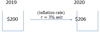
Assume that in 2019, you had a cart of groceries costs $200, and later in 2020, the same cart of groceries costs $206. Then,

$$ \frac{206}{200}=1.03 $$

Therefore, it implies that the cost of a cart of groceries grew by \(r=3% \)effective interest rate, which in this case is the inflation rate.

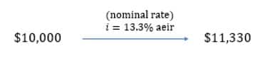
Consider also that you had in $10,000 in a separate investment account in 2019. Assume that this amount grows in such a way that it outpaces the inflation rate so that in 2020, the amount had grown to $11,330. Then,

$$ \frac{11,130}{10,000}=1.133 $$

Therefore, the amount grew by a nominal rate of \(i=13.3%\).

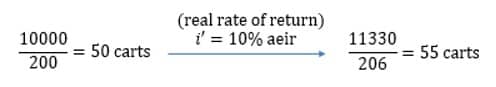
Now using both the basket of grocery example and the amount of funds in the investment account, we can illustrate the effect of inflation on the purchasing power.

In 2019, we had $10,000 and thus the number of carts of groceries you could buy at that time is:

$$ \frac{10000}{200}=50 \text{ carts} $$

And in 2020, the number of carts of groceries that could be bought is

$$ \frac{11330}{206}=55 \text{ carts} $$

Thus the ratio of the carts in 2020 to that in 2019 is:

$$ \frac{55}{50}=1.1 $$

Intuitively, the number of carts of groceries grew by \( {i}^\prime=10\% \) effective rate of interest. The rate of 10% is called the real rate of return since we have considered the effect of the inflation rate.

Therefore, using the above figures, we can relate the real rate of return, inflation rate, and the nominal rate. Working from the number of carts, we have that:

$$ \begin{align*} 55&=50\left(1+i^\prime\right)\Rightarrow \frac{11330}{206}=\frac{10000}{200}\left(1+i^\prime\right)\\ \therefore1+i&=(1+r)(1+i^\prime) \end{align*} $$

Example: Real Rate of Interest

A bank typically offers an effective rate of interest to be 7%. The economy is experiencing inflation of 3% in a given year.

Calculate the real rate of interest.

Solution

Accumulation of 1 for one year is equal to 1.07.

At the end of the year, 1.07 will only be worth:

$$ \frac{1.07}{1.03}=1.038835. $$

So the real rate of interest will be :

$$ 1.038835-1=0.038835=3.8835\% $$

Example: Inflation

A 40-year annuity due has annual payments of 6000. Assume a nominal interest rate of 8% compounded annually.

1. Determine the accumulated value of the annuity.
2. Assuming a 3% annual effective inflation rate, determine the accumulated value of the annuity using the real rate of return.
3. Determine the present value of the annuity by discounting the accumulated value in part (a) for 40 years using the inflation rate in part (b).

Solution

a. Determine the accumulated value of the annuity.

We need,

$$ 6000{\ddot{S}}_{\overline{40|}}@8\%=1,678,686 $$

b. Assuming a 3% annual effective inflation rate, determine the accumulated value of the annuity using the real rate of return.

Using the equation:

$$ (1+i)=(1+r)\cdot(1+i\prime) $$

we need to find the real rate of interest then:

$$ 1.08=(1.03)\cdot(1+i\prime)\Rightarrow i^\prime=0.0485 $$

And thus,

$$ 6000{\ddot{S}}_{\overline{40|}}@4.85\%=733,510 $$

c. Determine the present value of the annuity by discounting the accumulated value in part (a) for 40 years using the inflation rate in part (b).

We need,

$$ PV=1,678,686\cdot v_{0.03}^{40}=514,613 $$

Example: Inflation

As part of a settlement, Ed will receive a 20-year annual payment annuity, with the first payment equal to 1,000. Each subsequent payment will increase by an assumed annual inflation rate of 4%.

Determine the present value of this annuity, immediately before the first payment, using an annual effective interest rate of 7.12%.

Solution

Consider the following timeline:

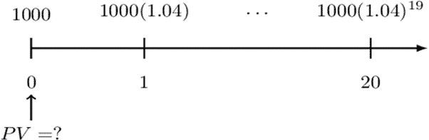
Clearly, we are dealing with a geometric annuity which is valued as follows:

Step 1: Value each payment at the Valuation Date

$$ PV=1000+1000\left(1.04\right)v+\cdots+1000\left(1.04\right)^{19}v^{19} $$

Step 2: Factor out the First Term

$$ PV=1000\left(1+\frac{1.04}{1.0712}+\cdots+\left(\frac{1.04}{1.0712}\right)^{19}\right) $$

Note that

$$ 1.0712=(1.03)(1.04) $$

And thus,

$$ PV=1000\left(1+\frac{1}{1.03}+\cdots+\left(\frac{1}{1.03}\right)^{19}\right) $$

Step 3: Recognize the Remaining Factor as \( {\ddot{a}}_{\overline{n|}} \text{ or } s_{\overline{n|}} \).

Looking at the expression in the parenthesis, it is easy to see that it is \( {\ddot{a}}_{\overline{20|}} \). Therefore,

$$ PV=1000\cdot{\ddot{a}}_{\overline{20|}.03}=15,324 $$

Note: In this question, we have r=0.04 and i=0.0712 so that the real rate of return is:

$$ 1+i=\left(1+r\right)\left(1+i^\prime\right)\Rightarrow i^\prime=\frac{1.0712}{1.04}-1=0.03 $$

Dollar-Weighted and Time-Weighted Rates of Return

These are rates used to measure the performance of a fund over a period of time—for example, funds of an insurance company.

This is important in order to differentiate between the money generated by the fund and the “new money,” otherwise there will be a threat of double counting or undercounting. New money is that extra money that was not generated by the fund itself. Note, however, that withdrawal from the money is equivalent to negative new money.

Dollar-Weighted Rate of Return (DWRR)

The dollar-weighted rate of return is a simple interest rate with an end of year valuation date where, for each transaction, time is measured from the date of the transaction until the end of the year. DWRR is also called the money-weighted rate of return.

DWRR is the rate of interest that satisfies the equation of value that includes the initial and the final fund values and the intermediate net cash flows. It important to understand once again that the dollar-weighted rate of return incorporates new money only; that is, the fund generated by the fund is totally ignored in the equation of value.

Unlike in an internal rate of return (IRR), the cash flows are accumulated in DWRR and equated to the final value of the fund. DWRR is defined as follows:

Consider a fund with an initial value of \( {B}_{0} \) at time 0, with the future cash flows \( {C}_{T} \) at time \( T=t_1,t_2,\ldots{1-t}_n,.., 1 \) ,denote the fund value at the end of the year by \( B_1 \) and the dollar weighted return by \( i_{DW}=i \), then the equation of value is given by:

$$ B_0(1+i)+C_{t_1}(1+t_1i)+C_{t_2}(1+t_2i)+\ldots+C_{{1-t}_n}(1+{(1-t}_n)i)=B_1 $$

Where \(i\) is the effective annual rate of interest earned by the fund in the time interval \([0,T]\).

Example: Calculating the Dollar-Weighted Rate of Return (DWRR)

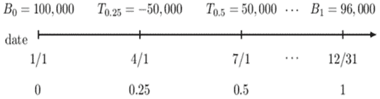
On January 1, an investment account has a balance of $100,000. On December 31, the balance is $96,000. You are given the following transaction information during the year:

$$ \begin{array}{c|c} \textbf{Date} & \textbf{Transaction} \\ \hline \text{April 1} & $ \text{50,000 withdrawal} \\ \hline \text{July 1} & $ \text{50,000 deposit} \end{array} $$

Determine the asset manager’s performance using a dollar-weighted rate of return.

Solution

Consider the following timeline:

The equation of value is:

$$ \begin{align*} &=100000\left(1+i\right)- 50000\left(1+0.75i\right)+ 50000\left(1+0.5i\right)\\ &=96000 \\ &=100000+100000i\pm 50000-50000\cdot0.75i+ 50000+50000\cdot0.5i\\ &=96000 \\ &\Rightarrow i\cdot\left(100000-50000\cdot0.75+50000\cdot0.5\right)\\ &=96000-100000+50000-50000 \end{align*} $$

The amount the parenthesis on the left-hand side of the last equation \((100000-50000∙0.75+50000∙0.5)\) above is termed as the exposure and the amount on the right-hand side \((96000-100000+50000-50000)\) is termed as the interest, and thus we can write:

$$ i\cdot(\text{Exposure})=\text{Interest} $$

Thus,

$$ i_{DW}=\frac{\text{Interest}}{\text{Exposure}}=\frac{96000-100000+50000-50000}{100000-50000\cdot0.75+50000\cdot0.5}=-0.0457 $$

Time-Weighted Rate of Return (TWRR)

The dollar-weighted rate of return is sensitive to both the amount of the cash flows and the timing. The time-weighted rate of return bypasses this disadvantage.

The time-weighted rate of return is a compound interest rate, which is determined by subtracting 1 from the annual accumulation factor. The annual accumulation factor is the product of the relevant periodic accumulation factors.

The idea behind the time-weighted rate of return is to calculate the growth factors between any two consecutive cash flows and then aggregates these factors (by finding the product) to come up with the overall rate of return for the whole length of time.

To compute the time-weighted rate of return, we need to calculate the rate of return in each subinterval between the transactions by comparing the fund balances just before a new transaction and the fund balance just after the last transactions.

Denote the fund value before and after the transaction at time \(j\) and \(j-1\) by \( B_j^B \) and \( B_{j-1}^A \), respectively. Also, denote the rate of return in a subinterval \(j-1\) to \( j \) by \(i_j\), then we have:

$$ 1+i_j=\frac{B_j^B}{B_{j-1}^A}, j=1, \ldots, n+1 $$

Denoting the TWRR by \( i_{TW} \), then:

$$ \begin{align*} 1+i_{TW}&=\prod_{j=1}^{n+1}{(1+i_j)}\\ \Rightarrow i_{TW}&=\left[\prod_{j=1}^{n+1}\left(1+i_j\right)\right]-1 \end{align*} $$

Since the time-weighted rate of return purges the effects of timing and amount of the cash flows, it is appropriate in measuring the performance of a fund manager.

Example: Calculating the Time-Weighted Rate of Return (TWRR)

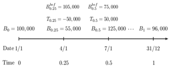
On January 1, an investment account has a balance of $100,000. On December 31, the balance is $96,000. You are given the following transaction information during the year:

$$ \begin{array}{c|c|c} \textbf{Date} &\textbf{Transaction}& \textbf{Balance before Transaction}\\ \hline \text{April 1} & $\text{50,000 withdrawal} &105,000\\ \hline \text{July 1} & $\text{50,000 deposit} &
75,000\end{array} $$

Determine the asset manager’s performance using a time weighted rate of return.

Solution

Consider the following timeline:

We know that,

$$ \begin{align*} i_{TW}&=\left[\prod_{j=1}^{n+1}\left(1+i_j\right)\right]-1 \\ &=\left[\frac{105000}{100000}\cdot\frac{75000}{55000}\cdot\frac{96000}{125000}\right]-1=0.0996 \\ \Rightarrow i_{TW}&=9.96\% \end{align*} $$

Alternatively, let:

$$ i_{TW}=i $$

Then,

$$ \begin{align*} 1+i&=aaf={paf}_0^{0.25}\cdot{paf}_{0.25}^{0.5}\cdot{paf}_{0.5}^1=\frac{105000}{100000}\cdot\frac{75000}{55000}\cdot\frac{96000}{125000}=1.0996 \\ \Rightarrow i&=0.0996 \end{align*} $$

Example: Typical Exam Question on Dollar- and Time-Weighted Rates of Return

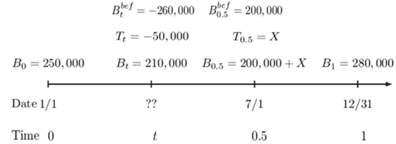
On January 1, an investment account has a balance of $250,000. On December 31, the balance is $280,000. You are given the following transaction information during the year:

$$ \begin{array}{c|c|c} \textbf{Date} & \textbf{Transaction} & \textbf{Balance before Transaction} \\ \hline \text{???} & \text{50,000 withdrawal} & {260,000} \\ \hline \text{July 1} & \text{X deposit} & {200,000} \end{array} $$

The exact date of the withdrawal is not known, but it is known to have taken place during the first half of the year. The dollar-weighted rate of return for the year is 11.4%, whereas the time-weighted rate of return for the year is 9.8%.

Determine the month in which the withdrawal occurred.

Solution

Consider the following timeline:

Now, let:

$$ i_{DW}=0.114=i $$

And

$$ i_{TW}=0.098=k $$

Then for the DWRR, we have:

$$ 250000\left(1+i\right)-50000\left(1+i\cdot\left(1-t\right)\right)+X\left(1+0.5i\right)=280000 $$

Also, for TWRR, we have:

$$ \begin{align*} 1+k&=\frac{260000}{250000}\cdot\frac{200000}{210000}\cdot\frac{280000}{200000+X}\Rightarrow\ \ 1.098=\frac{26}{25}\cdot\frac{20}{21}\cdot\frac{280000}{200000+X} \\ \therefore X&=52,580 \end{align*} $$

Going back to DWRR, we have:

$$ \begin{align*} &250000\left(1.114\right)-50000\left(1+0.114\cdot\left(1-t\right)\right)+52580\left(1+0.5(0.114)\right)\\ &=280000 \\ \Rightarrow t&=0.284 \text{ years after } \frac{1}{1}=3.4+(\text{months after } 1/1) \end{align*} $$

Thus, withdrawal occurred in April.

Duration and Convexity

Duration and convexity are the simple measures of the vulnerability of a portfolio to interest rate risk, where interest rate risk is the risk that arises from fluctuating interest rates. These measures assume a flat yield curve, which means that when the rates change, all other changes are equal.

Suppose that an institution has discounted assets of value V (A), which is supposed to meet the discounted liabilities V (L). If the interest rises, then both will decrease and vice versa. In order to examine these changes as the interest rates change, we use the changes in yield to maturity to represent changes in the underlying term structure.

Modified Duration

Modified duration expresses the change in the value of an asset or portfolio in response to a change in interest rates. Consider a series of cash flows of a portfolio \( C_t \) for all \( t=1,2,\ldots,n\). Let \(P\) be the present values of the payments at rate \(i\) (yield to maturity). Therefore:

$$ P(i)=\sum_{t=1}^{n}{C_tv^t } $$

The modified duration is defined to be:

$$ \begin{align*} \text{ModD}&=-\frac{1}{P(i)}\frac{dP(i)}{di}=-\frac{P^\prime(i)}{P(i)}\\ &=\left(\frac{1}{\sum_{t=1}^{n}{C_tv^t }}\right)\left(\sum_{k=1}^{n}{t.C_tv^{t+1}}\right)=\frac{\sum_{k=1}^{n}{t.C_tv^{t+1}}}{\sum_{t=1}^{n}{C_tv^t }} \end{align*} $$

It is important to note that the differentiation is done with respect to \(i\) and not \(v\) that is, if

$$ \begin{align*} P(i)&=\sum_{t=1}^{n}{{t\cdot C}_tv^t }=\sum_{k=1}^{n}{C_t{(1+i)}^{-t}\Rightarrow\frac{dP(i)}{di}=\sum_{k=1}^{n}{(-t)C_t\left(1+i\right)^{-t-1} }} \\ &=(-1)\sum_{k=1}^{n}{t.C_tv^{t+1} } \\ \Rightarrow-\frac{1}{P\left(i\right)}\frac{dP\left(i\right)}{di}&=-\frac{\left(-1\right)\sum_{k=1}^{n}{t.C_tv^{t+1}}}{\sum_{t=1}^{n}{C_tv^t}}=\frac{\sum_{k=1}^{n}{t.C_tv^{t+1}}}{\sum_{t=1}^{n}{C_tv^t }} \end{align*} $$

Modified duration is always positive, and it measures the percentage decrease of the value of the investment per unit increase in the yield to maturity.

Macaulay Duration

Just as modified duration, Macaulay duration is also a measure of portfolio sensitivity to the interest rate. Macaulay duration is defined as the average of the term of cash flows \( (C_t) \) weighted by the present value and expressed as the number of payments periods. In other words, the Macaulay duration of a set of payments is the weighted average of the times of the payments, where the weight of the payment at time \(t\) is equal to the present value of the payment at time t divided by the present value of all the payments. 

Consider the following timeline:

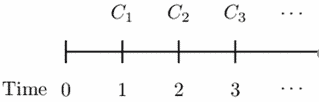
By definition,

$$ \begin{align*} \text{MacD}&=\frac{1\cdot C_1\cdot v+{2\cdot C}_2\cdot v^2+{3\cdot C}_3\cdot v^3+\cdots}{C_1\cdot v+C_2\cdot v^2+C_3\cdot v^3+\cdots}\\ &=\frac{\sum{{t\cdot C}_tv^t}}{\sum{C_t\cdot v^t}} \end{align*} $$

Note that factoring out \((1+i)\) in the numerator of the above equation then:

$$ \begin{align*} \text{MacD}&=\frac{(1+i)\sum_{t=1}^{n}{tC_tv^{t+1} }}{\sum_{t=1}^{n}{C_tv^t }}=\left(1+i\right) \text{ModD} \\ \Rightarrow \text{MacD}&=\text{ModD}\left(1+i\right)\Longleftrightarrow \text{ModD}=\text{MacD}\cdot v \end{align*} $$

The Macaulay duration of a bond that pays an annual coupon of \(D\) and redeemed at \(R\) is given by:

$$ \text{MacD}=\frac{D\left(Ia\right)_{\overline{n|}}+Rnv^n}{Da_{\overline{n|}}+Rv^n} $$

If it is a zero-coupon bond of the nominal amount of $100 then,

$$ \text{MacD}=\frac{100nv^n}{100v^n}=n $$

This is obvious since the mean term of equal payments must be the time of that cash flow.

Example: Macaulay Duration

Calculate the Macaulay Duration of a bond redeemable at par in 10 years that has an annual coupon of 8% and an interest rate of 10% per annum.

Solution

$$ \begin{align*} \text{MacD}&=\frac{D\left(Ia\right)_{\overline{n|}}+Rnv^n}{Da_{\overline{n|}}+Rv^n} \\ &=\frac{8\left(Ia\right)_{\overline{10|}}+10\times100v^{10}}{8a_{\overline{10|}}+100v^{10}}=\frac{617.83}{87.71}=7.04 \text{ years} \end{align*} $$

Duration of a Portfolio of Assets

The duration of a portfolio of assets equals the weighted average of the duration of the assets that form the portfolio, with the weight associated with the duration of an individual asset being the ratio of the price of that asset to the price of the portfolio.

Consider a portfolio with three assets A, B, and C. Then,

$$ \begin{align*} \text{MacD}_{pf}&=\frac{\left(\sum{{t\cdot C}_t\cdot v^t}\right)_{Pf}}{\left(\sum{C_t\cdot v^t}\right)_{Pf}}\\ &=\frac{\left(\sum{{t\cdot C}_t\cdot v^t}\right)_A+\left(\sum{{t\cdot C}_t\cdot v^t}\right)_B+\left(\sum{{t\cdot C}_t\cdot v^t}\right)_C}{P_{Pf}}\\ &=\frac{\left(\sum{{t\cdot C}_t\cdot v^t}\right)_A}{P_{Pf}}+\frac{\left(\sum{{t\cdot C}_t\cdot v^t}\right)_B}{P_{Pf}}+\frac{\left(\sum{{t\cdot C}_t\cdot v^t}\right)_C}{P_{Pf}}\\ &=\frac{P_A}{P_{Pf}}\cdot\frac{\left(\sum{{t\cdot C}_t\cdot v^t}\right)_A}{P_A}+\frac{P_B}{P_{Pf}}\cdot\frac{\left(\sum{{t\cdot C}_t\cdot v^t}\right)_B}{P_B}+\frac{P_C}{P_{Pf}}\cdot\frac{\left(\sum{{t\cdot C}_t\cdot v^t}\right)_C}{P_C}\\ &=\frac{P_A}{P_{Pf}}\cdot\left(MacD\right)_A+\frac{P_B}{P_{Pf}}\cdot\left(MacD\right)_B+\frac{P_C}{P_{Pf}}\cdot\left(MacD\right)_C \end{align*} $$

Note that

$$ P_{Pf}=P_A+P_B+P_C $$

Example: Duration of a Portfolio of Assets

A portfolio of assets has three types of bonds with the following characteristics:

Bond A has a price of 2,000 and a Macaulay duration of 9.5

Bond B has a price of 3,000 and a Macaulay duration of 9.0

Bond C has a price of 5,000 and a Macaulay duration of 16.0

All prices and Macaulay durations above were calculated using an annual effective interest rate of 6%.Determine the Macaulay duration of the portfolio using an annual effective interest rate of 6%.

Solution

We have:

$$ \begin{align*} P_{Pf}&=P_A+P_B+P_C \\ &=2000+3000+5000 \\ &=10000 \end{align*} $$

Then,

$$ \text{MacD}_{pf}=\frac{2000}{10000}\left(9.5\right)+\frac{3000}{10000}\left(9.0\right)+\frac{5000}{10000}\left(16.0\right)=12.6 $$

Convexity

Convexity is a measure of the curvature in the relationship between the price and yield of a bond. Whereas duration is the first derivative of the price of the bond with respect to interest rates, convexity is the second derivative of the price of the bond with respect to interest rates. Graphically, it can be represented as follow:

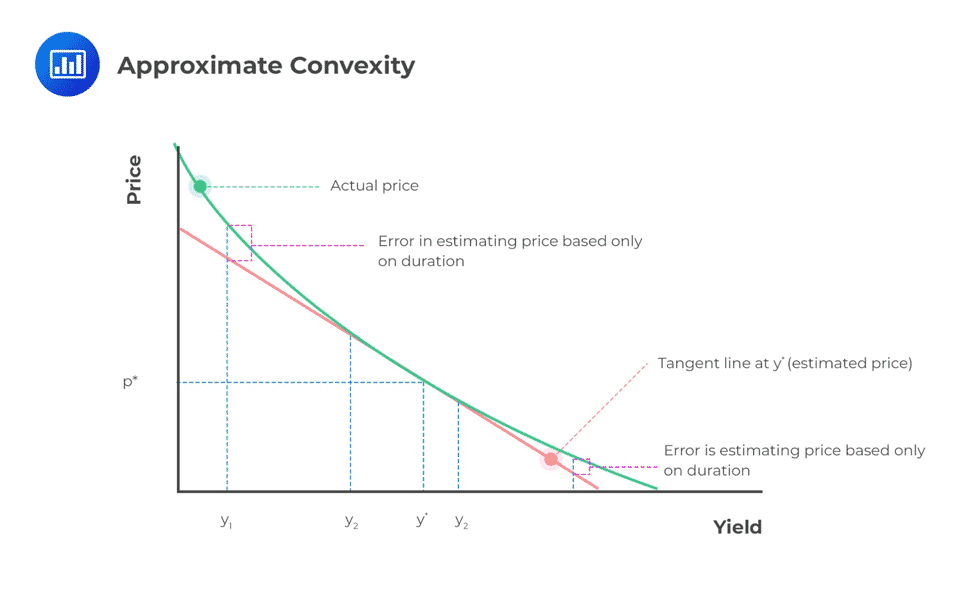Convexity determines precisely the effect of interest changes on a portfolio by giving a measure of the change in the duration of a bond when the interest rate changes. It implies that (\P\) increases when there is a decrease in the interest rate and increases when there is the same level in the interest rate.

Definition: The Macaulay convexity of a set of payments is the weighted average of the squares of the times of the payments, where the weight assigned to the payment at time t is equal to the present value of the payment at time t divided by the present value of all the payments. Macaulay convexity is defined as:

$$ MacC=\frac{1^2\cdot C_1\cdot v+{2^2\cdot C}_2\cdot v^2+{3^2\cdot C}_3\cdot v^3+\cdots}{C_1\cdot v+C_2\cdot v^2+C_3\cdot v^3+\cdots}=\frac{\sum{{t^2\cdot C}_t\cdot v^t}}{\sum{C_t\cdot v^t}} $$

On the other hand, modified convexity is defined as:

$$ \begin{align*} \text{ModC}&=\frac{1}{P}\frac{d^2}{di^2}P=\frac{P^{\prime\prime}(i)}{P(i)}\\ &=\left(\frac{1}{\sum{C_t\cdot v^t}}\right)\left(\sum{t\left(t+1\right)C_tv^{t+2}}\right)=\frac{\sum{t\left(t+1\right)C_tv^{t+2}}}{\sum{C_t\cdot v^t}} \end{align*} $$

Convexity is always positive.

Example: Modified and Macaulay Convexities

Consider the following the payments presented by the following timeline.

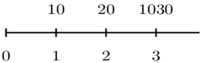
For the set of payments above, using i=0.06, determine

1. the Macaulay convexity, and
2. the modified convexity.

a)

$$ \begin{align*} \text{MacC}&=\frac{\sum{{t^2\cdot C}_t\cdot v^t}}{\sum{C_t\cdot v^t}}\\ &=\frac{1^2\cdot10\cdot v+2^2\cdot20\cdot v^2+3^2\cdot1030\cdot v^3}{10\cdot v+20\cdot v^2+1030\cdot v^3}\\ &=8.815 \end{align*} $$

b)

$$ \begin{align*} \text{ModC}&=\frac{\sum{t\left(t+1\right)C_tv^{t+2}}}{\sum{C_t\cdot v^t}}\\ &=\frac{20\cdot\left(1+i\right)^{-3}+120\cdot\left(1+i\right)^{-4}+12360\cdot\left(1+i\right)^{-5}}{10\cdot\left(1+i\right)^{-1} +20\cdot\left(1+i\right)^{-2}+1030\cdot\left(1+i\right)^{-3}}\\ &=\frac{9,347.95}{892.04}=10.48 \end{align*} $$

Example: Modified Convexity

An annuity pays $X forever from a lump sum deposited in a bank account for an infinite term that pays a simple interest i at a constant rate at the end of each year.

Find the expression of modified convexity.

Solution

$$ \begin{align*} P(i)&=Xa_{\overline{\infty|}}=\frac{X}{i} \\ c\left(i\right)&=\frac{1}{P\left(i\right)}\frac{d^2}{di^2}P(i)=\frac{P^{\prime\prime}(i)}{P(i)}=\frac{\frac{2X}{i^3}}{\frac{X}{i}}=\frac{2}{i^2} \end{align*} $$

First Order Approximations

1st Order Approximation Based on Modified Duration

Using modified duration and convexity, we can approximate change in the present value P(i) (which in this case can be a price of a bond) as follows:

Let \( \Delta i=i_{new}-i_{old} \) be the change in the rate of interest. Then using the Taylor series expansion and using modified duration only, then:

$$ \begin{align*} \Rightarrow P\left(i+\Delta i\right)&=P\left(i\right)+\frac{dP\left(i\right)}{di}\epsilon_i \\ &=P\left(i\right)\left[1-\left(-\frac{1}{P\left(i\right)}\frac{dP\left(i\right)}{di}\right)\Delta_i\right] \end{align*} $$

Since,

$$ \begin{align*} \text{ModD}&=-\frac{1}{P(i)}\frac{dP(i)}{di}\\ \Rightarrow P\left(i+\Delta i\right)&=P\left(i\right)\left[1-\text{ModD}.\Delta_i\right] \end{align*} $$

Clearly, the change in price \( \Delta P(i) \) is

$$ \begin{align*} \Delta P\left(i\right)&=-P\left(i\right).\text{ModD}.\Delta_i\\ \Rightarrow P\left(i+\Delta i\right)&=P\left(i\right)-\Delta P\left(i\right) \end{align*} $$

We also know that,

$$ \text{ModD}=\text{MacD}\cdot v $$

Thus, we can write,

$$ \begin{align*} P\left(i+\Delta i\right)&=P\left(i\right)\left[1-ModD.\Delta_i\right]\\ &=P\left(i\right)\left[1-MacD\cdot v.\Delta_i\right]\\ &=P\left(i\right)-P\left(i\right).MacD\cdot v.\Delta_i\\ \Rightarrow\Delta P\left(i\right)&=-P\left(i\right).MacD\cdot v.\Delta_i \end{align*}$$

1st Order Based on Macaulay Duration

If we use Macaulay duration only, we have:

$$ ∆P(i)=P(i)∙\left[\left( \cfrac{1+i_\text{old}}{1+i_\text{new}}\right)^\text{MacD}-1\right] $$

So,

$$ P\left(i+\Delta i\right)=P\left(i\right)-∆P(i) $$

Note that,

$$ P\left(i\right)=P\left(i_{old}\right) $$

And

$$ \Delta i=i_\text{new}-i_\text{old} $$

Example: First Order Approximations based on Modified and Macaulay Durations

A bond has a price of 7025 to yield 7% annual effective. Using this same yield rate, the Macaulay duration of the bond is 4.95 years. Determine the price of the bond to yield 6.5% annual effective, using

1. the first-order modified approximation, and
2. the first-order Macaulay approximation.

Solution

1. Since we are given Macaulay duration, we have

   $$ \begin{align*} P\left(i+\Delta i\right)&=P\left(i\right)\left[1-\text{ModD}.\Delta_i\right]\\ &=P\left(i\right)\left[1-\text{MacD}\cdot v.\Delta_i\right] \\ &=P\left(i\right)-P\left(i\right).\text{MacD}\cdot v.\Delta_i \\ P\left(0.065\right)&=P\left(0.07\right)-P\left(0.07\right).\frac{4.95}{1.07}. (0.07-0.065)\\ &=7025-7025\cdot\frac{4.95}{1.07}\cdot(0.065-0.07) \\ &=7025+162=7187 \end{align*} $$

2. Macaulay duration first approximation is given:

   $$ \begin{align*} \Delta P&=P(i).\left[\left( \cfrac{1+i_{old}}{1+i_{new}}\right)^ \text{MacD}-1 \right] \\ &=7025\cdot\left[\left(\frac{1.07}{1.065}\right)^{4.95}-1\right]=165 \\ \Rightarrow P\left(0.065\right)&=7025+165=7190 \end{align*} $$

Special Case Duration Shortcut

Consider an n-year annual coupon bond, redeemable at par, and bought to yield an annual effective interest rate that is equal to the coupon rate as shown by the following timeline,

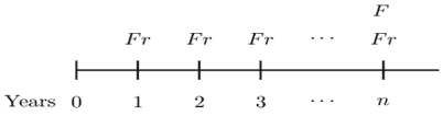
The Macaulay and modified durations can be shown to be:

$$ \text{MacD}={\ddot{a}}_{\overline{n}|} $$

And

$$ \text{[ModD}=\text{MacD} \cdot v=a_{\overline{n}|} $$

Similarly, consider an n-year monthly coupon bond, redeemable at par, is bought to yield a monthly effective interest rate that is equal to the monthly effective coupon rate,

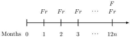
The Macaulay and modified durations are given by:

$$ \text{MacD}={\ddot{a}}_{\overline{12n}|} $$

And

$$ \text{ModD}= \text{MacD} \cdot v=a_{\overline{12n}|} $$

Consider the following example:

Example: Special Case Duration Shortcut

A 20-year annual coupon bond, redeemable at par, is bought to yield an annual effective interest rate that is equal to the coupon rate. Determine an expression for the Macaulay duration of the bond.

Solution

We know that:

$$ \text{MacD}=\frac{\sum{{t\cdot C}_tv^t}}{\sum{C_t\cdot v^t}} $$

So, in this case, we have,

$$ \begin{align*} \text{MacD} &=\frac{1\cdot F r\cdot v+2\cdot F r\cdot v^2+\ldots+20\cdot F r\cdot v^{20}+20\cdot F\cdot v^{20}}{Fr\cdot a_{\overline{20}|}+F\cdot v^{20}}\\ &=\frac{Fr\cdot\left(Ia\right)_{\overline{20}|}+20\cdot F\cdot v^{20}}{Fr\cdot a_{\overline{20}|}+F\cdot v^{20}}\\ &=\frac{r\cdot\left(Ia\right)_{\overline{20}|}+20\cdot v^{20}}{r\cdot a_{\overline{20}|}+v^{20}}\\ &=\frac{r\cdot\left[\frac{{\ddot{a}}_{\overline{20}|}-20v^{20}}{i}\right]+20\cdot v^{20}}{r\cdot\left[\frac{1-v^{20}}{i}\right]+v^{20}} \end{align*} $$

Now since, i=r, we have

$$ \text{MacD}=\frac{r\cdot\left[\frac{{\ddot{a}}_{\overline{20}|}-20v^{20}}{i}\right]+20\cdot v^{20}}{r\cdot\left[\frac{1-v^{20}}{i}\right]+v^{20}}=\frac{{\ddot{a}}_{\overline{20}|}-20v^{20}+20\cdot v^{20}}{1-v^{20}+v^{20}}={\ddot{a}}_{\overline{20}|} $$

Which proves our result. Also, note that,

$$ \text{ModD}=\text{MacD}\cdot v=v.{\ddot{a}}_{\overline{20}|}=a_{\overline{20}|} $$

 

Yield Rate

An interest is referred to as a yield rate or the internal rate of return (IRR) if it gives the return an investor can earn from an investment. In other words, it equates the present value of cash inflows to zero.

Assume a project which exists for n years has future cashflows denoted by \( C_1,{C}_2,\ldots,{C}_n \) and denote IRR by i then we have:

$$ \sum_{k=1}^{n}{C_k\left(1+i\right)^{-k}}=\sum_{k=1}^{n}{C_kv^{-k}}=0 $$

This equation can also be written as:

$$ C_0=-\sum_{k=1}^{n}{C_kv^{-k}} $$

This implies that the net present value of the future cash inflows evaluated at a yield rate is equal to the initial cash outlay.

Example: Yield Rate

A project requires a startup of $2,000. It is expected that the investment will earn $800 at the end of the first year and $1,600 after 2 years at will end its transactions. Calculate the internal rate of return of the project.

Solution

We know that

$$ \begin{align*} \sum_{k=1}^{n}{C_kv^{-k}}&=0 \\ \Rightarrow-2000+800v+1600v^2&=0 \\ =4v^2+2v-5&=0 \end{align*} $$

Use the Quadratic formula:

$$ \begin{align*} x&=\frac{-b\pm\sqrt{b^2-4ac}}{2a}. \text{ Where } a=4, b=2, c=-5 \text{ and } x=v \\ \Rightarrow v&=\frac{-2\pm\sqrt{4+80}}{8}=-1.3956 \text{ or } 0.89564 \\ \therefore v&=0.89564\Rightarrow\left(1+i\right)^{-1}=0.895664 \end{align*} $$

So,

$$ i=\left(0.895664 \right)^{-1}-1=0.1165=11.65\% $$

The above example is a case where the equation of value can be solved directly using common mathematical principles, to find the yield rate. There is the case where there are more than two cash flows.

It is worth noting that IRR is used in project appraisal. For instance, if the IRR is the same as the effective rate at which bank transaction is done, then the investment is favorable.

The Term Structure of Interest Rates

The interest rate that applies to most investments varies with the term (time) of the investment. This phenomenon is termed as the term structure of interest rates. In other words, rates of interest differ according to the time period of the term of investment, which is, in general, \(i_s\neq i_t\) for all \(s\neq t\), this phenomenon is called the term structure of interest rates, and its corresponding graph of spot rates is called the yield curve.

Yield curves are generally increasing and concave down. If all spot rates are equal, then the yield curve is flat. Until now, the whole course has assumed a flat yield curve (which we have been assuming all along). Conversely, if long-term rates are less than short-term rates, then the yield curve is inverted.

Spot Rates and Forward Rates

Spot Rates

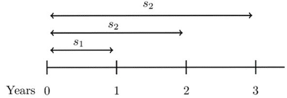
Spot rate can be defined as the annual effective interest earned by funds invested now for a period of time. As such, for t>0 define the spot rate by \( s_t. \) Consider the following table

$$ \begin{array}{c|c} \textbf{Length of Investment} & \textbf{Interest Rate} \\ \hline \text{1 year} & {7.00\%} \\ \hline \text{2 years} & {8.00\%} \\ \hline \text{3 years} & {8.75\%} \\ \hline \text{4 years} & {9.25\%} \\ \hline \text{5 years} & {9.50\%} \end{array} $$

All rates shown are annual effective interest rates. Today’s rates, as shown in the table, are called spot rates. Therefore,

$$ s_1=7\%, s_2=8\% \cdots $$

Consider the following timeline:

From the timeline, it is easy to see that:

$$ aaf_0^1=1+s_1\Rightarrow adf_1^0=\left(1+s_1\right)^{-1}= v_1 \\ paf_0^2=\left(1+s_2\right)^2\Rightarrow ppf_2^0=\left(1+s_2\right)^{-2}=v_2^2 \\ ppf_0^3=\left(1+s_3\right)^3\Rightarrow ppf_3^0=\left(1+s_3\right)^{-3}=v_3^3 $$

Note that aaf = annual accumulation factor, adf= annual discount factor, paf= periodic accumulation factor and pdf= periodic discount factor.

Forward Rates

A forward rate is an effective rate of interest that is applicable to financial transactions that will take place in the future. We can relate the spot rates and forward rates.

Consider the following timeline:

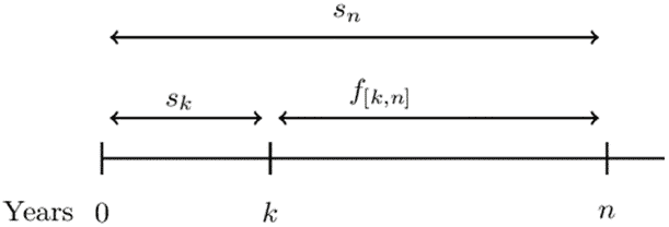
\( f_{\left[k,n\right]} \) denotes the forward rate from time k to time n and it is the annual effective interest rate used to accumulate or discount between times k and n.

It is easy to note that,

$$ \begin{align*} aaf_0^n&=aaf_0^k\cdot aaf_k^n \\ \Rightarrow\left(1+s_n\right)^n&=\left(1+s_k\right)^k.\left(1+f_{\left[k,n\right]}\right)^{n-k} \\ \therefore\left(1+f_{\left[k,n\right]}\right)^{n-k}&=\frac{\left(1+s_n\right)^n}{\left(1+s_k\right)^k} \end{align*} $$

Example: Spot Rates and Forward Rates

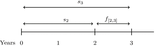
Consider the following annual effective rates (spot rates).

$$ \begin{array}{c|c} \textbf{Length of Investment} & \textbf{Interest Rate} \\ \hline \text{1 year} & {7.00\%} \\ \hline \text{2 years} & {8.00\%} \\ \hline \text{3 years} & {8.75\%} \\ \hline \text{4 years} & {9.25\%} \\ \hline \text{5 years} & {9.50\%} \end{array} $$

Determine the forward rate from year 2 to year 3

Consider the following timeline:

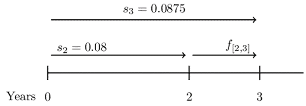
So,

$$ \begin{align*} \left(1+s_3\right)^3&=\left(1+s_2\right)^2\cdot1+f[2,3] \\ \Rightarrow\left(1.0875\right)^3&=\left(1.08\right)^2\cdot\left(1+f_{\left[2,3\right]}\right)\\ \therefore f_{\left[2,3\right]}&=\frac{\left(1.0875\right)^3}{\left(1.08\right)^2}=0.10265=10.3\% \end{align*} $$

Alternatively, we can use the formula above so that:

$$ \begin{align*} \left(1+f_{\left[2,3\right]}\right)^{3-2}&=\frac{\left(1+s_3\right)^3}{\left(1+s_2\right)^2}\\ \Rightarrow1+f_{\left[2,3\right]}&=\frac{\left(1.0875\right)^3}{\left(1.08\right)^2}=1.1027 \\ \therefore f_{\left[2,3\right]}&=0.10265=10.3\% \end{align*} $$

Spot Rates, Forward Rates, and Zero-Coupon Bonds

Spot rates are mostly based on zero-coupon bonds. As such, spot rates are also termed as zero-coupon rates. Assume a zero-coupon bond of the term \( \textbf{n} \) (say) with an issue price, \( \textbf{P}_\textbf{n} \).

Discrete Time Spot Rates

The yield on a unit zero-coupon bond is called n-year spot rate of interest denoted by \( s_n \). It is the measure of mean interest rate from now until the end of n- years The equation of value of a unit zero-coupon bond will be:

$$ P_n=\left(1+s_n\right)^{-n}\Rightarrow\left(1+s_n\right)=P_n^{-\frac{1}{n}} $$

Also note that:

$$ \left(1+s_n\right)^n=v^{-n} $$

Example: Discrete-Time Spot Rate

Calculate the one-year spot rate of a zero-coupon bond priced at $94 per $100 nominal.

Solution

$$ P_n=\left(1+s_n\right)^{-n} \\ \Rightarrow100\left(1+s_n\right)^{-1}=94\therefore s_n=\left(\frac{94}{100}\right)^{-1}=0.06382=6.82% $$

The yield curve can also represent the redemption yields meaning it is not necessarily the spot rates.

Discrete-time Forward Rates

The discrete forward which can be denoted by \( f_{\left[k,n\right]} \) is the yearly rate of interest, which is agreed upon at time 0 for an investment made at time k>0 for a period of n-k years.

For example, an investor agrees to invest $50 at time k for n-k years then accumulated amount at time n is:

$$ 50(1+f_{\left[k,n\right]}) $$

Briefly, the forward rate of interest \( f_{k,n} \) measures the mean interest rate between times k and n.

There is, however, the connection between the spot rates and forward rates. The accumulation amount at time k of investment of 1 at time t=0 is given by \( \left(1+s_k\right)^k\).If we had agreed to invest this amount at time k for n-k years so that the accumulation at time n will be:

$$ \left(1+s_k\right)^k.\left(1+f_{\left[k,n\right]} \right) $$

We are also aware that 1 invested at time 0 for n years will be

$$ \left(1+s_n\right)^n $$

Note also that the price of a zero-coupon bond of 1 invested for n years accumulates to \( P_n^{-n} \)

$$ \Rightarrow\left(1+s_k\right)^k.\left(1+f_{\left[k,n\right]} \right)=\left(1+s_n\right)^n=P_n^{-n} $$

From this, we get the following relationship:

$$ \left(1+f_{\left[k,n\right]}\right)^{n-k}=\frac{\left(1+s_n\right)^n}{\left(1+s_k\right)^k}=\frac{P_k}{P_n} $$

From these relationships, it is clear that the full term structure of interest rate may be determined by the given spot rates and forward rates.

For a one-period rate, \( f_k=f_{k,1} \) . Also, define \(f_0=s_1\) . Using the same arguments,

$$ \Rightarrow\left(1+s_n\right)^n=\left(1+f_0\right)\left(1+f_1\right)\left(1+f_2\right)\ldots(1+f_{n-1}) $$

The one-year forward rate \( f_t=f_{t,1} \) is the rate in the time interval (k,k+1) and can represented as:

$$ 1+f_t=\frac{\left(1+s_{k+1}\right)^{k+1}}{\left(1+s_k\right)^k} $$

Example: Forward Rates

Given that 6%, 5.7%, and 5% are the 3, 5 and 7-year spot rates per year respectively and that the forward rate from time 4 is 5.2% per year, find f[5,7]

Solution

We are given \(s_3=6\%, s_5=5.7\% s_7=5\%, f[3,7]=5.2\% \)

We know that

$$ \begin{align*} \left(1+f_{\left[k,n\right]} \right)^{n-k}&=\frac{\left(1+s_n\right)^n}{\left(1+s_k\right)^k}=\frac{P_k}{P_n} \\ \Rightarrow \left(1+f_{\left[2,3\right]} \right)&=\frac{\left(1+s_n\right)^3}{\left(1+s_k\right)^2}=\frac{P_2}{P_3}=\frac{940}{910} \\ f_{\left[2,3\right]}&=\frac{94}{91}-1=0.03296=3.30\% \end{align*} $$

Example: Spot Rates, Forward Rates, and Zero-Coupon Bonds

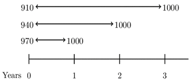
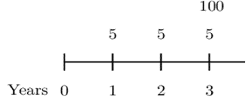
You are given the following prices for 1000 par value zero-coupon bonds:

$$ \begin{array}{c|c} \textbf{Duration} & \textbf{Price} \\ \hline \text{1 year} & {970} \\ \hline \text{2 years} & {940} \\ \hline \text{3 years} & {910} \end{array} $$

Determine the forward rate from time 2 to time 3 that corresponds to these prices.

Solution

Consider the following timeline:

We know that,

$$ \begin{align*} \left(1+f_{\left[k,n\right]} \right)^{n-k}&=\frac{\left(1+s_n\right)^n}{\left(1+s_k\right)^k}=\frac{P_k}{P_n} \\ \Rightarrow \left( 1+f[2,3] \right)&=1+sn31+sk2=P2P3=940910 \\ \Rightarrow f[2,3]&=\frac{94}{91}-1=0.03296=3.30\% \end{align*} $$

Alternatively, we can use the fact that:

$$ \left(1+s_n\right)^n=v^{-n} $$

Consider the following timeline:

It is easy to see that:

$$ \left(1+s_3\right)^3=\left(1+s_2\right)^2\cdot\left(1+f[2,3]\right) \\ v_3^{-3}=v_2^{-2}\cdot1+f[2,3] $$

From the tables, we know that,

$$ 940=1000v_2^2\Rightarrow v_2^2=0.94 $$

And

$$ \begin{align*} 910&=1000v_3^3\Rightarrow v_3^3=0.910 \\ \Rightarrow{0.91}^{-1}&={0.94}^{-1}\cdot\left(1+f_{\left[2,3\right]}\right)\Rightarrow f_{\left[2,3\right]}=\frac{94}{91}-1=0.03296=3.30\% \end{align*} $$

Example: Implied Yield on Coupon Bonds

You are given that the annual yield on zero-coupon bonds with a duration of k years is \(i_k\)=0.03+0.005(k-1).

Determine the annual yield rate for a 3-year bond with 5% annual coupons that are consistent with this term structure of interest rates.

Solution

From the annual yield function, we have that:

$$ s_1=i_1=0.030, s_2=i_2=0.035 \text{ and } s_3=i_3=0.040 $$

Now, consider the following timeline:

Then the equation of value is:

$$ \begin{align*} 5\cdot v_1&+5\cdot v_2^2+105v_3^3=5\cdot a_{\overline{3}|i}+100v_i^3 \\ \Rightarrow\frac{5}{1.03}&+\frac{5}{{(1.035)}^2}+\frac{105}{{(1.04)}^3}=5\cdot a_{\overline{3}|i}+100v_i^3 \\ \therefore5\cdot a_{\overline{3}|i}&+100v_i^3=102.866\Rightarrow i=0.03967=3.97\% \end{align*} $$

Therefore, the yield curve defined by the \( i_k=0.03+0.005(k-1) \) on a 3-year bond implies an annual rate of 3.97%.

Continuous-Time Spot Rates

The continuous-time spot rate is defined as the force of interest that is equivalent to an effective rate of interest rate, which corresponds to the spot rate. Like in discrete-time spot rate, let \( P_n \) be the price of a unit zero-coupon bond with the term n-years. Then,

$$ P_n=e^{-\left(\delta_nn\right)}\Rightarrow\delta_n=-\frac{1}{n}\ln{P_n} $$

Where \( \delta_n \) is the n-year spot force of interest. It is also called the continuously compounded spot rate of interest or the continuous-time spot rate.

The n-year spot force of interest is connected to the corresponding discrete-time spot rate \(s_n\) just like i and \(\delta\) that is,1+i= \(e^\delta\). Similarly, to spot rates,

$$ 1+s_n=e^{\delta_n}\Rightarrow s_n=e^{\delta_n}-1 $$

Continuous-Time Forward Rates

Denote continuous-time forward rate of interest from time k to n by \(F_{[k,n]}\). It is defined as the force of interest equivalent to the annual forward interest \(f_{[k,n]}\). If $1 is invested for n-k years starting at time k which is agreed at time \( 0 \le k \) accumulates to \( \left(1+f_{\left[k,n\right]}\right)^{n-k} \) at time n using the annual forward rates \(f_{\left[k,n\right]}\). Now, applying the equivalent forward force of interest, the same investment will accumulate to

$$ e^{(n-k)F[k,n]} $$

Therefore, the relationship is given by:

$$ f_{[k,n]}=e^{(n-k)F[k,n]}-1 $$

Now consider the investment of $1 at time 0 using the spot rate \(\delta_k\) for k years and then followed by forward rates \(F[k,n]\). This is similar to the investment of $1 at a continuous-time spot rate \(\delta_n\) for n years. Therefore:

$$ \begin{align*} e^{k\delta_k}e^{(n-k)F_{[k,n]}}]&=enδn\\ \Rightarrow k\delta_k+(n-k)F_{[k,n]}&=nδn\\ \therefore F_{[k,n]}&=\frac{n {\delta_n}-k {\delta_k}}{n-k} \end{align*} $$

Now using the relation \( \delta_n=-\frac{1}{n}\ln{P_{n }} \) then, the above equation reduces to (the algebra is trivial)

$$ \begin{align*} F[k,n]&=\frac{(n)-\frac{1}{n}lnP_n -(k).-\frac{1}{k}lnP_k} {n-k} \\ &=\frac{1}{n-k}\left[\ln{P_k}-\ln{P_n}\right] \\ \therefore F[k,n]&=\frac{1}{n-k}ln\left[\frac{P_k}{P_n}\right] \end{align*} $$

Example: Continuous Forward Rates

The prices for the zero-coupon bonds at various years are as follows:

1 year=94%, 5 years=70%, 10 years=47%, 15 years=30%.

Calculate the continuous-time forward rates between year 5 and year 15.

Solution

We know that

$$ \begin{align*} F_{[k,n]}&=\frac{1}{n-k}ln\left[\frac{P_k}{P_n}\right] \\ \Rightarrow F_{[5,15]}&=\frac{1}{10}ln(\frac{P5}{P15})=\frac{1}{10}ln(\frac{70}{30})=0.08473=8.473\% \end{align*} $$

Stock Valuation

Stock represents the share in the company’s ownership and translates to claim in the company’s earnings and assets. Hence one will receive dividends from the earnings annually.

The stock price is the discounted value of all dividends received. The general formula for stock valuation is given by:

$$ \text{PV of stock}=\sum_{t=1}^{\infty}\frac{D_t}{\left(1+r\right)^t} $$

\( D_t\) is the dividend received at any time t and r is the required rate of return.

Dividend Discount Model

This is a technique used to calculate the stock price of a company based on the assumption that the stock price is equal to the sum of the present value of all future dividends received.

There are many forms of this model. For instance:

1. If it is assumed that all future dividends will be equal, then the present value of these dividends is equivalent to perpetuity. Given the required rate of return is r then the price of a stock will be;

   $$ P_0=\frac{D}{r} $$

2. If there is a constant dividend growth rate g, then the price of a stock will be in the form of growing perpetuity. The stock price will be given by:

   $$ P_0=\frac{D}{1+r}+\frac{D(1+g)}{\left(1+r\right)^2}+\frac{D\left(1+g\right)^2}{\left(1+r\right)^3}+\ldots \\ =\frac{D}{r-g} $$

Example: Price of a Stock with Equal Dividends

A company’s common stock presently pays $1.00 as a dividend, which is expected to remain at this rate forever. The required rate of return is 10%.

Calculate the price of the stock today.

Solution

$$ P_0=\frac{D}{r}=\frac{1}{0.1}=$10 $$

Example: Price of a Stock with Dividend Growth Rate

Consider two stocks A and B. Both stocks are valued using the discount model, and their dividends are paid annually on the same date. The dividend growth rate for stock A is g, and that of B is -g. The price of stock A is twice that of B at a 6% rate of return.

Calculate g.

Solution

We know that the price of a stock

$$ P=\frac{D}{r-g} $$

Where

D= amount of divided

r= rate of return

g= dividend growth rate

Therefore,

$$ P_A=\frac{D}{r-g} $$

And

$$ P_B=\frac{D}{r+g} $$

From the information we know that:

$$ \begin{align*} P_A&=2P_B \\ \Rightarrow\frac{D}{0.06-g}&=2\left(\frac{D}{0.06+g}\right)\Rightarrow g=2\% \end{align*} $$