


Solvency, Liquidity and Other Regulati ...
After completing this reading, you should be able to: Describe and calculate the... Read More
After completing this reading, you should be able to:
Value-at-Risk (VaR) accounts for leverage and portfolio diversification, thus providing a measure of risk based on the current positions. In this section, we will discuss the different VaR measures associated with portfolio construction.
A portfolio is composed of various asset positions. We can construct a portfolio VaR based on a combination of risks of the underlying assets.
Assume that an investor can invest in any of N securities, \(i=1,2,…, N\), and a proportion \({ \text{w} }_{ \text{i} }\) is invested in security \(i\), the portfolio return \({ \text{R} }_{ \text{p} }\) can be expressed as a random variable which is a linear combination of random variables, \({ \text{R} }_{ \text{i} }\), representing security \(i\)’s return so that:
$$ { \text{R} }_{ \text{P} } = \sum _{ \text{i}=1 }^{ \text{N} }{ { \text{w} }_{ \text{i} }{ \text{R} }_{ \text{i} } } $$
This means that the portfolio return is simply the weighted average of the individual security returns.
Note:
\({ \text{w} }_{ \text{i} }\) is a proportion of the total sum to be invested:
$$ \sum _{ \text{i=1} }^{ \text{N} }{ { \text{w} }_{ \text{i} } } =1, $$
The portfolio’s expected return is given by:
$$ \text{E} \left( \text{R}_{\text{p}} \right)={ \mu }_{\text{p}}=\sum _{ \text{i=1} }^{ \text{N} }{ { \text{w} }_{ \text{i} }{ \mu }_{ \text{i} }} $$
And the portfolio’s variance is:
$$ \begin{align*} \text{VaR}\left( { \text{R} }_{ \text{p} } \right) & ={ \sigma }_{ \text{p} }^{ 2 }=\sum _{ \text{i}=1 }^{ \text{n} }{ { \text{w} }_{ \text{i} }^{ 2 }{ \sigma }_{ \text{i} }^{ 2 } } +\sum _{ \text{i}=1 \\ \text{j}=1 }^{ \text{N} }{ \sum _{ \left( \text{j}\neq 1 \right) }^{ \text{N} }{ { \text{w} }_{ \text{i} }{ \text{w} }_{ \text{j} }{ \sigma }_{ \text{ij} } } } \\ & = \sum _{ \text{i}=1 }^{ \text{N} }{ { \text{w} }_{ \text{i} }^{ 2 }{ \sigma }_{ \text{i} }^{ 2 } }+2 \sum _{ \text{i}=1 }^{ \text{N} }{ \sum _{ \left( \text{j} < 1 \right) }^{ \text{N} }{ { \text{w} }_{ \text{i} }{ \text{w} }_{ \text{j} }{ \sigma }_{ \text{ij} } } } \end{align*} $$
The sum above accounts for both the risk of the individual securities \({ \sigma }_{ \text{i} }^{2}\) and the covariances which sum to \( \frac {\text{N}\left(\text{N}-{1}\right)}{2}\) different terms. The portfolio variance will be lower when the correlations are lower. This is a general result – if we have enough independent securities, the variation of a portfolio of these assets approaches zero.
We aim to obtain a VaR measure from the portfolio variance. If we assume the individual security returns to be normally distributed, the portfolio return, which is a linear combination of jointly normal random variables, will also have a normal distribution. We can then translate the confidence level \(c\) into a Z-Score denoted by \(α\) such that the probability of the existence of a loss worse than \(–α\) is equal to \(c\). Thus with \(w\) as the initial portfolio value, the portfolio VaR is given by:
$$ \text{Portfolio VaR}= \text{VaR}_{ \text{P} }= \alpha { \sigma }_{ \text{P} } { \text{W} }={ \alpha } \sqrt{ { \text{x} }^{ \prime }\sum { \text{x} } } $$
Where \(x\) represents the vector of dollar amount invested in each asset.
As the number of securities N making up the portfolio gets very large, the contribution to the portfolio variance of the variances of the individual securities goes to zero. The individual risk of securities can be diversified away.
We can thus define diversified VaR as the VaR incorporating diversification benefits between securities.,
The fundamental formula for diversified VaR is similar to the portfolio VaR given by:
$$ { \text{VaR} }_{ \text{p} }= \alpha \times { \sigma }_{ \text{p} } \times \text{W} $$
Where:
\({ \alpha }\) is the standard normal deviate relating to the confidence level \(c\);
\({ \sigma }_{ \text{p} }\) is the volatility of the portfolio return; and
\(W\) is the nominal amount invested in the portfolio.
A portfolio is made up of two foreign currencies, USD and EUR. The currencies have a volatility of 5% and 10%, respectively, relative to the dollar. Assume that the portfolio has US$4 million invested in the USD and US$3 million in EUR.
At a 95% confidence level, determine the diversified portfolio VaR assuming that the positions are uncorrelated.
$$\sum\ x=\left[\begin{matrix}{0.05}^2&0\\0&{0.12}^2\\\end{matrix}\right]\left[\begin{matrix}$4\\$3\\\end{matrix}\right]=\left[\begin{matrix}{0.05}^2\times$4+0\times$3\\0\times$4+{0.10}^2\times$3\\\end{matrix}\right]=\left[\begin{matrix}$0.01\\$0.03\\\end{matrix}\right]$$
Note on matrix multiplication: The first step of matrix multiplication shown above is to multiply the rows of the first matrix by the columns of the second matrix. If you need further explanation on how to do this, refer to the chapter’s video lesson by Prof. James Forjan.
$$\sigma_p^2\ =[\begin{matrix}$4&$3]\\\end{matrix}\left[\begin{matrix}$0.01\\$0.03\\\end{matrix}\right]=0.04+0.09=0.13$$
$$ \text{Dollar volatility} = \sqrt(0.13)=$0.360555 \text{ million}$$
At 95% confidence level, α=1.65,
$$VaR_p=1.65\times$0.360555\ million=$594,916$$
Individual VaR is the VaR of individual security in isolation. The individual risk of each security is given by:
$$ { \text{VaR} }_{ \text{i} }=\alpha { \sigma }_{ \text{i} }\left| { \text{w} }_{ \text{i} } \right| =\alpha { \sigma }_{ \text{i} }\left| { \text{w} }_{ \text{i} } \right| \text{W} $$
Where:
\({ \text{w} }_{ \text{i} }\) is the portfolio weight invested in security \(i\).
\({ \text{W} }_{ \text{i} }\) is the nominal amount invested in security \(i\).
\(W\) is the portfolio value.
The absolute value of the weight \( \text{w}_{ \text{i} }\) is used because it can be negative. However, the risk measure must be a positive value.
Summing individual VaRs of two perfectly correlated securities gives the portfolio VaR.
A given portfolio is made up of two perfectly correlated assets, M and N. The volatility of asset M is 10% while that of asset N is 12%. The nominal amount invested in asset M is $1 million, while that invested in asset N is $0.8 million.
Calculate the individual VaR of assets M and N at the 95 percent confidence level.
$$ {\text{VaR}}_{\text{i}}= \alpha { \sigma }_{ \text{i} } { \text{w} }_{ \text{i} } $$
The individual VaRs will be
$$ \begin{align*} {\text{VaR}}_{\text{M}}&=1.65\times0.10\times$ 1,000,000=$ 165,000 \\ {\text{VaR}}_{\text{N}}&=1.65\times0.12\times$ 800,000=$ 158,400 \end{align*} $$
Marginal VaR is defined as the additional amount of risk that new security adds to an existing portfolio.
Consider an existing portfolio, with N securities and \(j=1,2,…, N\); we can obtain a new portfolio by adding a unit of protection. The sensitivity of the portfolio volatility to a change in weight is given by:
$$ \cfrac { { \delta \sigma }_{ \text{p} } }{ { \delta \text{w} }_{ \text{i} } } =\cfrac { \text{cov}\left( { \text{R} }_{ \text{i} },{ \text{R} }_{ \text{p} } \right) }{ { \sigma }_{ \text{p} } } $$
Thus, we can express the marginal VaR as a vector component given by:
$$ \Delta { \text{VaR} }_{ \text{i} }=\cfrac { { \delta }\text{VaR} }{ { \delta \text{x} }_{ \text{i} } } =\cfrac { { \delta }\text{VaR} }{ { \delta \text{w} }_{ \text{i} }\text{W} } =\alpha \cfrac { \text{cov}\left( { \text{R} }_{ \text{i} },{ \text{R} }_{ \text{p} } \right) }{ { \sigma }_{ \text{p} } } $$
Note that the marginal VaR is unitless.
The marginal VaR is related to the beta, which is defined as:
$$ { \beta }_{ \text{i} }=\cfrac { \text{cov}\left( { \text{R} }_{ \text{i} },{ \text{R} }_{ \text{p} } \right) }{ { \sigma }_{ \text{p} }^{ 2 } } =\cfrac { { \sigma }_{ \text{ip} } }{ { \sigma }_{ \text{p} }^{ 2 } } =\cfrac { { \rho }_{ \text{ip} }{ \sigma }_{ \text{i} }{ \sigma }_{ \text{p} } }{ { \sigma }_{ \text{p} }^{ 2 } } =\cfrac { { \rho }_{ \text{ip} }{ \sigma }_{ \text{i} } }{ { \sigma }_{ \text{p} } } $$
Beta measures the amount of risk that one security contributes to total portfolio risk. The beta can be estimated from the slope coefficient in a regression of \({ \text{R} }_{ \text{i} }\) and \({ \text{R} }_{ \rho }\), simply expressed as:
$$ { \text{R} }_{ \text{i} }={ \alpha }_{ \text{i} }+{ \beta }_{ \text{i} } { \text{R} }_{ \text{p} }+{ \epsilon }_{ \text{i,t} } $$
The vector beta can be written in matrix form as:
$$ \beta = \cfrac { \sum \text{w} } { \text{w}^{‘} \sum \text{w}} $$
The relationship that exists between the marginal VaR (\( \Delta { \text{VaR} }\)) and beta (\({ \beta }\))is expressed by:
$$ \Delta { \text{VaR} }_{ \text{i} }=\cfrac { { \delta }\text{VaR} }{ { \delta \text{x} }_{ \text{i} } } \alpha \left( { \beta }_{ \text{i} }\times { \sigma }_{ \text{p} } \right) =\cfrac { \text{VaR} }{ \text{W} } \times { \beta }_{ \text{i} } $$
Consider a portfolio M which has three equally weighted securities 1, 2, and 3. Each security has a value of $100,000. Assume that the portfolio VaR is $20,000.
Given that security 2 has a beta of 1.5, calculate the marginal VaR of security 2.
Using the formula:
$$ \text{Marginal VaR} \left( \Delta { \text{VaR} }_{ \text{i} } \right)=\cfrac { { \delta }\text{VaR} }{ { \delta \text{x} }_{ \text{i} } } \alpha \left( { \beta }_{ \text{i} }\times { \sigma }_{ \text{p} } \right) =\cfrac { \text{VaR} }{ \text{W} } \times { \beta }_{ \text{i} } $$
W is the value of the portfolio = \( 100,000 \times 3=$300,000 \)
$$ { \beta }_{2}=1.5 $$
Thus,
$$ \Delta {\text{VaR}}_{2}=\cfrac { \text{VaR} }{ \text{W} } \times { \beta }_{ \text{i} }= \cfrac {20,000} {300,000} \times 1.5=0.1 $$
This implies that a one-dollar change in the value of security 2 causes a 0.1 change in the portfolio VaR.
Incremental VaR gauges the impact of small changes in individual assets on the total VaR. It is different from marginal VaR in that it tells us the exact amount of risk added or subtracted from the entire portfolio, while marginal VaR gives an estimation of the risk amount.
We can evaluate the total impact of a proposed trade on a portfolio. Let \(a\) be a vector of new positions. The portfolio VaR is measured at the initial position \( {\text{VaR}}_{\text{p}} \) and at the new position \( \text{VaR}_{{\text{p}}+{\text{a}}} \). The incremental VaR is then expressed as:
$$ \text{Incremental VaR} = \text{VaR}_{{\text{p}}+{\text{a}}} – \text{VaR}_{\text{p}} $$
A decrease in VaR implies that the new trade is risk-reducing; otherwise, it is risk-increasing.
The shortcoming of this approach it is time-consuming since it requires a full revaluation of the portfolio VaR with a new trade.
When \( \text{VaR}_{\left( \rho \right)+\text{a}} \) is expanded in series around the origin, we have:
$$ \text{VaR}_{\text{p}+\text{a}}= \text{VaR}_{\text{p}}+\left( \Delta \text{VaR} \right)^{\prime } \times {\text{a}}+ \dots $$
The second-order terms can be ignored if the deviation is small. Hence, incremental VaR can be approximated as:
$$ \text{Incremental VaR} \approx \left( \Delta \text{VaR} \right)^{\prime } \times \text{a} $$
This measure is simple to use because \( \Delta {\text{VaR}} \) is a by-product of the initial computation \({\text{VaR}}_{\text{p}}\).
Incremental VaR is useful where a trade involves a set of new exposures to the risk factors. For instance, in a case where the risk factor involved is only one, the portfolio value changes from W to \( \text{W}_{{\text{p}}+{\text{a}}}={{\text{W}}+{\text{a}}} \) , with \(a\) as the amount invested in asset \(i\). The variance of the dollar return on the portfolio is then given by:
$$ { \sigma }_{ \text{p}+\text{a} }^{ 2 }{ { \text{w} }_{ \text{p}+\text{a} }^{ 2 } }={ \sigma }_{ \text{p} }^{ 2 }{ \text{w} }^{ 2 }+2\text{aw}{ \sigma }_{ \text{ip} }+{ \text{a} }^{ 2 }{ \sigma }_{ \text{i} }^{ 2 } $$
If we differentiate it with respect to \(a\), we get:
$$ \cfrac { { \delta }{ \sigma }_{ \text{p}+\text{a} }^{ 2 }{ { \text{w} }_{ \text{p}+\text{a} }^{ 2 } } }{ { \delta }\text{a} } =2\text{w}{ \sigma }_{ \text{ip}+2\text{a}{ \sigma }_{ \text{i} }^{ 2 } } $$
This leads to a zero value for:
$$ { \text{a} }^{*} = – \cfrac {\text{w}{ \sigma }_{ \text{ip} }}{{ \sigma }_{ \text{i} }^{ 2 }}= – \cfrac{\text{w}{ \beta }_{ \text{i} }{ \sigma }_{ \text{p} }^{ 2 }}{{ \sigma }_{ \text{i} }^{ 2 }} $$
Where \({ \text{a} }^{*}\) is the variance-minimizing position. The variance-minimizing position or the best hedge is the additional amount invested in an asset to reduce the underlying portfolio risk.
Consider a portfolio composed of two foreign currencies, namely USD and EUR. Assume that these currencies are uncorrelated and have volatility against the dollar of 5% and 10%, respectively. The portfolio has US$4 million invested in the USD and US$3 million in EUR.
At a 95% confidence level, find the incremental VaR given that the USD currency increases by US$15,000.
Using the marginal VaR approach, \({ \beta }\) can be obtained, such that:
$$ \begin{align*} \beta & = \cfrac { \sum \text{w} } { \text{w}^{\prime} \sum \text{w}} = \text{W} \times \cfrac { \sum \text{x} } { \text{x}^{\prime} \sum \text{x}} \\ \text{W} & =$4+$3=$7 \\ \sum { \text{x} } &= \left[ \begin{matrix} { 0.05 }^{ 2 } \\ 0 \end{matrix}\begin{matrix} 0 \\ { 0.10 }^{ 2 } \end{matrix} \right] \left[ \begin{matrix} $4 \\ $3 \end{matrix} \right] =\left[ \begin{matrix} \left( { 0.05 }^{ 2 }\times $4 \right) +\left( { 0 }\times $3 \right) \\ \left( { 0 }\times $4 \right) +\left( { 0.10 }^{ 2 }\times $3 \right) \end{matrix} \right] =\left[ \begin{matrix} 0.01 \\ 0.03 \end{matrix} \right] \\ { \text{x} }^{ \prime }\sum { \text{x} } & = \left[ $4\quad $3 \right] \left[ \begin{matrix} 0.01 \\ 0.03 \end{matrix} \right] =\left( $4\times 0.01 \right) +\left( $3\times 0.03 \right) =0.13 \\ \text{Dollar volatility} & = \sqrt{0.13}=0.360555 \\ \end{align*} $$
Therefore,
$$ \beta = $7 \times \cfrac {\left[ \begin{matrix} $0.01 \\ $0.03 \end{matrix} \right] } {0.13} = $7 \times \left[ \begin{matrix} 0.0769 \\ 0.2308 \end{matrix} \right] =\left[ \begin{matrix} 0.5383 \\ 1.6154 \end{matrix} \right] $$
We then find the marginal VaR by:
$$ \Delta { \text{VaR} }=\alpha \cfrac { \text{cov}\left( { \text{R} },{ \text{R} }_{ \rho } \right) }{ { \sigma }_{ \text{p} } } =1.65 \times \cfrac {\left[ \begin{matrix} $0.01 \\ $0.03 \end{matrix} \right] } {\sqrt{0.13}} = 1.65 \left[ \begin{matrix} 0.0277 \\ 0.0832 \end{matrix} \right] = \left[ \begin{matrix} 0.045705 \\ 0.13728 \end{matrix} \right] $$
With an increment of $15,000 in the first position, the incremental VaR becomes:
$$ \left( \Delta \text{VaR} \right)^{\prime} \times {\text{a} } = \left[ 0.045705\quad 0.13728 \right] \left[ \begin{matrix} $15,000 \\ 0 \end{matrix} \right] =$685.58 $$
Moreover, we can compare this with the incremental VAR obtained from a full revaluation of the portfolio risk. An addition of $15,000 to the first position leads to:
$$ \begin{align*} { \sigma }_{ \text{p}+\text{a} }^{ 2 }{ { \text{w} }_{ \text{p}+\text{a} }^{ 2 } }&=\left[ $4.015\quad $3 \right] \left[ \begin{matrix} { 0.05 }^{ 2 } \\ 0 \end{matrix}\begin{matrix} 0 \\ { 0.1 }^{ 2 } \end{matrix} \right] \left[ \begin{matrix} $4.015 \\ $3 \end{matrix} \right] =\left[ 4.015\quad 3 \right] \left[ \begin{matrix} 0.0100375 \\ 0.030000 \end{matrix} \right] \\ 0.04030056+0.09&=$0.13030056 \text{ million} \\ \text{VaR}_{ \text{p}+\text{a} }&=1.65 \times \sqrt{$0.130301}=$595,603 \end{align*} $$
Finally, we can compute the exact increment by finding the difference of the initial \({\text{VaR}}_{\text{p}}\) and \({\text{VaR}}_{\text{p}+\text{a}}\), i.e.,
$$ \begin{align*} {\text{VaR}}_{\text{p}}&=1.65\times \sqrt{0.13}=$594,916 \\ \text{VaR}_{\text{p}+\text{a}}-\text{VaR}_{ \text{p} }&=$595,603-$594,916 =$687 \end{align*} $$
From the above calculations, we note that the \(\Delta \text{VaR}\) approximation of $686 is very close to the true value, $687.
For a risk to be managed, it is important to decompose the risk of the current portfolio. We require the additive decomposition of VaR that takes into account the power of diversification. In this case, the marginal VaR will be the guiding tool in measuring the contribution of each asset to the existing portfolio risk.
To obtain the component VaR, we multiply the marginal VaR by the current dollar position in the risk factor \(i\). This can be expressed mathematically as:
$$ \begin{align*} \text{Component} \text{ VaR}_{ \text{i} }&=\left( \Delta \text{VaR}_{ \text{i} } \right) \times \text{w}_{ \text{i} } \text{W} \\ &= \cfrac {\text{VaR} {\beta}_{\text{i}}} {\text{w}} \times \text{w}_{ \text{i} } \text{W}= \text{VaR} { \beta }_{ \text{i} } \text{w}_{ \text{i} } \end{align*} $$
The component VaR shows how the portfolio VaR varies if the element was removed from the collection. When VaR components are small, the quality of linear approximation improves. This implies that the decomposition is more important with large portfolios, which have many small positions.
The total VaR can be expressed as a sum of component VaRs. That is,
$$ \text{CVaR}_{1}+\text{CVaR}_{2}+⋯+\text{CVaR}_{\text{N}}=\text{VaR}\left( \sum _{ \text{i}=1 }^{ \text{N} }{ { \text{w} }_{ \text{i} }{ \beta }_{ \text{i} } } \right) = \text{VaR} $$
Where:
\(\sum _{ \text{i}=1 }^{ \text{N} }{ { \text{w} }_{ \text{i} }{ \beta }_{ \text{i} } } = 1\) which is the beta of the portfolio with itself.
Since \( { \beta }_{ \text{i} } = { \rho }_{ \text{i} } \times \cfrac {{ \sigma }_{ \text{i} }}{{ \sigma }_{ \rho }} \) , the component VaR can be written as:
$$ \text{CVaR}_{\text{i}}=\text{VaR} { \text{w} }_{ \text{i} }{ \beta }_{ \text{i} } = \left(\alpha { \sigma }_{ \text{p} } \text{W} \right) { \text{w} }_{ \text{i} }{ \beta }_{ \text{i} } = \left(\alpha { \sigma }_{ \text{i} } \text{W}_{\text{i} } \text{W} \right)_{\text{pi}}=\text{VaR}_{\text{iPi}} $$
This can then be normalized by the total portfolio VaR to give:
$$ \% \text{ contribution to VaR of component i}= \cfrac {\text{CVaR}_{\text{i}}} {\text{VaR}} ={ \text{w} }_{ \text{i} }{ \beta }_{ \text{i} } $$
Consider portfolio M which has three equally weighted securities 1, 2, and 3. Each security has a value of $100,000. Assume that the portfolio VaR is $20,000.
Given that security 2 has a beta of 1.5, calculate the component VaR of security 2.
Using the formula:
$$ {\text{CVaR}_{\text{i}}}=\text{VaR} { \text{w} }_{ \text{i} }{ \beta }_{ \text{i} } $$
VaR=$20,000
\({ \beta }_{2}\)=1.5
\({ \text{w} }_{2}= \cfrac {100,000} {300,000}\)
Thus,
$$ \text{CVaR}_{2}=20,000 \times \cfrac {1}{3} \times 1.5=$10,000 $$
$10,000 is the amount that the portfolio VaR will decrease if security 2 is eliminated.
The portfolio VaR of two perfectly correlated assets is equal to the sum of the individual VaRs. When correlation is equal to 1, \(\text w_1\) and \(\text w_2\) are positive. The sum of individual VaRs when the correlation coefficient is unity is referred to as an undiversified portfolio VaR.
It is given by:
$$ { \text{VaR} }_{ \text{p} }={ \text{VaR} }_{1}+{ \text{VaR} }_{2} $$
A given portfolio is made up of two perfectly correlated assets, M and N. The volatility of asset M is 10%, while that of asset N is 12%. The nominal amount invested in asset M is $1 million, while asset N is $0.8 million.
Calculate the portfolio VaR at the 95 percent confidence level.
$$ \text{VaR}_{\text{p}}= \sum_{\text{i}} { \text{VaR}_{ \text{i} }} $$
We then compute the individual VaR as \( { \text{VaR} }_{ \text{i} }= \alpha { \sigma }_{ \text{i} } { \text{x} }_{ \text{i} } \)
$$VaR_M=1.65\times0.10\times$\ 1,000,000=$\ 165,000$$
$$VaR_N=1.65\times0.12\times$\ 800,000=$\ 158,400$$
$$VaR_P=$165,000+$158,400=$323,400$$
The most precise measure of linear dependence between variables is the correlation coefficient, which is given by:
$$ { \rho }_{12}= \cfrac {\text{COV}_{12}} {{\sigma}_{1}{ \sigma }_{2} } $$
Where:
\( { \text{COV} }_{12} \) is the covariance between securities 1 and 2; and
\( { \sigma }_{ \text{i} } \) is the standard deviation of security \(i\).
Typically, the correlation coefficient \(\rho\) lies between -1 and 1. A correlation coefficient of unity implies that the variables have a perfect linear relationship, and if equal to -1, the variables are said to have a perfectly negative relationship. A correlation of 0 implies that the variables are not correlated.
In a portfolio consisting of two assets, the standard deviation of the portfolio is expressed by:
$$ { \sigma }_{ \text{p} }^{ 2 }={ \text{w} }_{ \text{i} }^{ 2 }{ \sigma }_{ \text{i} }^{ 2 }+{ \text{w} }_{ 2 }^{ 2 }{ \sigma }_{ 2 }^{ 2 }+{ 2\text{w} }_{ 1 }{ \text{w} }_{ 2 }{ \rho }_{ 12 }{ \sigma }_{ 1 }{ \sigma }_{ 2 } $$
Thus, the portfolio VaR is given by:
$$ \text{VaR}_{ \text{P} }=\alpha { \sigma }_{ \rho } \text{W}= \alpha \sqrt { { \text{w} }_{ 1 }^{ 2 }{ { \sigma }_{ 1 }^{ 2 }+{ \text{w} }_{ 2 }^{ 2 }{ \sigma }_{ 2 }^{ 2 }+{ 2\text{w} }_{ 1 }{ \text{w} }_{ 2 }{ \rho }_{ 12 }{ \sigma }_{ 1 }{ \sigma }_{ 2 }} } \text{W} $$
In cases where the correlation coefficient is 0, the portfolio VaR reduces to:
$$ \text{VaR}_{ \text{P} }=\sqrt { { { \alpha }^{ 2 }\text{w} }_{ 1 }^{ 2 }{ \text{w} }_{ 2 }^{ 2 }{ \sigma }_{ 1 }^{ 2 } } =\sqrt { { \text{VaR} }_{ 1 }^{ 2 }+{ \text{VaR} }_{ 2 }^{ 2 } } $$
If the correlation is ±1 and \( \text{w}_{1} \) and \( \text{w}_{2} \) are both positive, the portfolio VaR equation reduces to:
$$ \begin{align*} \text{VaR}_{ \text{P} } \left( \text{Undiversified portfolio} \right) & = \sqrt { { \text{VaR} }_{ 1 }^{ 2 }+{ \text{VaR} }_{ 2 }^{ 2 } + 2 \text{VaR}_{ 1 } \times \text{VaR}_{ 2 } } \\ & =\text{VaR}_{ 1 } + \text{VaR}_{ 2 } \end{align*} $$
The portfolio VaR is equivalent to the sum of the individual VaR measures if the two assets are perfectly correlated. The difference between the diversified VaR and the undiversified VaR gives the benefit of diversification. Therefore, the undiversified VaR provides the portfolio with VaR when there is no short position, and all correlations are 1.
Portfolio VaR can be 0 in case the correlation is -1 between, for example, two assets. However, undiversified VaR creates an upper bound on VaR in the sense that if the correlation between those two assets moves over time from -1 to +1, then our previous estimate of portfolio VaR is wrong. The upper bound should be \( \text{VaR}_{1} \) +\( \text{VaR}_{2} \) , or the undiversified VaR, which does not account for the correlation between the assets.
We can conclude that the undiversified VaR gives the upper bound on the portfolio VaR in case the correlations are unstable and, at the same time, move in the wrong direction. This is the worst-case scenario for the portfolio.
A portfolio manager computes the VaR for two assets in her portfolio:
\( \text{VaR}_{1} = $4 \text{ million } \)
\( \text{VaR}_{2} = $3 \text{ million } \)
Assuming that the returns of the two assets are perfectly correlated, calculate the VaR of the portfolio.
Since the two assets are perfectly correlated,
$$ \begin{align*} \text{VaR}_{ \text{p} }&=\text{VaR}_{1}+\text{VaR}_{2} \\ &=$4+$3=$7 \text{ million} \end{align*} $$
Generally, lower portfolio risk is attained from low correlations and a large number of assets. To see the impact of portfolio size (N) on the VaR, we assume that all assets have the same risk, correlations are the same, and equal weight is placed on each asset.
Portfolio risk decreases as the number of assets increases. Diversifiable risk tends to zero asymptotically as illustrated in the following graph:
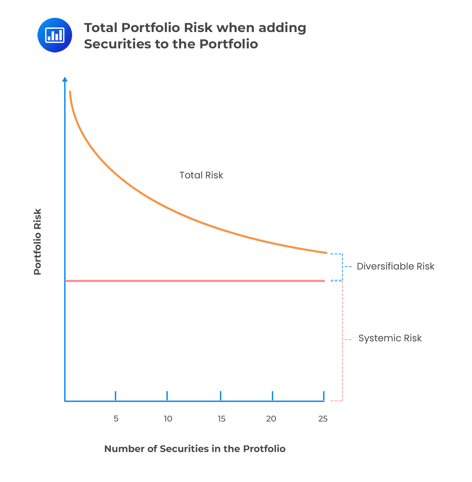 Portfolio risk is given by:
$$ { \sigma }_{ \rho }= \sigma \sqrt {\left( \cfrac { 1 }{ \text{N} } \right) +\left( 1-\cfrac { 1 }{ \text{N} } \right) { \rho } } $$
As N becomes larger, the portfolio risk tends to \(\sigma \sqrt{ \rho }\).
The covariance between independent assets is zero. As N increases, the variance of the portfolio approaches zero. In other words, lower risk can be achieved by diversification. Generally, the correlation coefficient and the covariance between assets is positive.
Investment returns tend to move together, i.e., they are positively correlated. Thus, the contribution to the portfolio variance of the variances of the individual assets tends to zero as N grows. However, the contribution of the covariance components approaches the average covariance as N gets large. Thus, the individual risk of positions can be diversified away, but the contribution to the total risk caused by the covariance terms cannot be diversified away.
A portfolio is made of 10 assets. Each asset has a value of $3 million.
Given that the volatility for each asset is 20%, and the correlation between any two returns is 0.3, calculate the portfolio VaR assuming a Z-value of 1.96.
Portfolio risk is given by:
$$ \begin{align*} { \sigma }_{ \rho }&= \sigma \sqrt {\left( \cfrac { 1 }{ \text{N} } \right) +\left( 1-\cfrac { 1 }{ \text{N} } \right) { \rho } } \\ &= 0.20 \times \sqrt { \cfrac { 1 }{ 10 } +\left( 1-\cfrac { 1 }{ 10 } \right) \times 0.3 } =0.1217 \end{align*} $$
Thus,
$$ \begin{align*} \text{VaR}_{ \text{P} }&=\alpha \times { \sigma }_{\text{p}} \times {\text{P}} \\ &=1.96\times0.1217\times10\times$3 \text{ million} =$7.156 \text{ million} \end{align*} $$
Risk management deals with risk and ways of minimizing the risk. However, reducing the risk does not always generate the optimal portfolio. On the other hand, portfolio management requires gauging both risks and return measures to choose the optimal portfolio.
Marginal VaR can be applied to risk management. If the investor has the choice to reduce all positions by fixed amounts and aims to lower the portfolio VaR, he/she should rank all marginal VaR values and select the asset with the largest marginal VaR. This is because it will have the greatest hedging effect.
Using our earlier example, we can show how to employ marginal VaRs to make decisions to lower the risk of the entire portfolio.
Consider a portfolio composed of two foreign currencies, namely the USD and EUR. Assume that these currencies are uncorrelated and have volatility against the dollar of 5% and 10%, respectively. The portfolio has US$4 million invested in the USD and US$3 million in EUR.
At a 95% confidence level, find the incremental VaR given that the USD currency increases by US$15,000.
Using the marginal VaR approach, \({ \beta }\) can be obtained, such that:
$$ \begin{align*} \text{W}&=$4+$3=$7 \\ \sum { \text{x} }&= \left[ \begin{matrix} { 0.05 }^{ 2 } \\ 0 \end{matrix}\begin{matrix} 0 \\ { 0.10 }^{ 2 } \end{matrix} \right] \left[ \begin{matrix} $4 \\ $3 \end{matrix} \right] =\left[ \begin{matrix} \left( { 0.05 }^{ 2 }\times $4 \right) +\left( { 0 }\times $3 \right) \\ \left( { 0 }\times $4 \right) +\left( { 0.10 }^{ 2 }\times $3 \right) \end{matrix} \right] =\left[ \begin{matrix} 0.01 \\ 0.03 \end{matrix} \right] \\ { \text{x} }^{ \prime }\sum { \text{x} }&= \left[ $4\quad $3 \right] \left[ \begin{matrix} 0.01 \\ 0.03 \end{matrix} \right] =\left( $4\times 0.01 \right) +\left( $3\times 0.03 \right) =0.13 \\ \text{Dollar volatility} &= \sqrt{0.13}=0.360555 \\ \text{VaR}_{ \text{P} }&=1.65 \times \sqrt{0.13}=$594,916 \end{align*} $$
Assume that the amount invested in USD is increased to $5 million and that in EUR is reduced to $2 million. The portfolio variance will be:
$$ \begin{align*} \text{W}&=$5+$2=$7 \\ \sum { \text{x} }&= \left[ \begin{matrix} { 0.05 }^{ 2 } \\ 0 \end{matrix}\begin{matrix} 0 \\ { 0.10 }^{ 2 } \end{matrix} \right] \left[ \begin{matrix} $5 \\ $2 \end{matrix} \right] =\left[ \begin{matrix} \left( { 0.05 }^{ 2 }\times $5 \right) +\left( { 0 }\times $2 \right) \\ \left( { 0 }\times $5 \right) +\left( { 0.10 }^{ 2 }\times $2 \right) \end{matrix} \right] =\left[ \begin{matrix} 0.0125 \\ 0.02 \end{matrix} \right] \\ { \text{x} }^{ \prime }\sum { \text{x} }&= \left[ $5\quad $2 \right] \left[ \begin{matrix} 0.0125 \\ 0.02 \end{matrix} \right] =\left( $5\times 0.0125 \right) +\left( $2\times 0.02 \right) =0.1025 \\ \text{VaR}_{ \text{P} }&=1.65 \times \sqrt{0.1025}=$528,258 \end{align*} $$
Notice that VaR of $528,258 is less than the VaR of $594,916, generated when the USD portfolio has a lower weight. The marginal VaRs should be much closer in value:
$$ \left[ \begin{matrix} \text{cov}\left( { \text{R} }_{ \text{USD} },{ \text{R} }_{ \text{P} } \right) \\ \text{cov}\left( { \text{R} }_{ \text{EUR} },{ \text{R} }_{ \text{P} } \right) \end{matrix} \right] =\left[ \begin{matrix} { 0.05 }^{ 2 } \\ 0 \end{matrix}\begin{matrix} 0 \\ { 0.10 }^{ 2 } \end{matrix} \right] \left[ \begin{matrix} $5 \\ $2 \end{matrix} \right] =\left[ \begin{matrix} 0.0125 \\ 0.02 \end{matrix} \right] $$
As predicted, 0.02 and 0.0125 are closer in value than 0.01 and 0.03.
The marginal VaRs of the two positions are calculated as follows:
$$ \begin{align*} \Delta { \text{VaR} }_{ \text{USD} }&=\alpha \cfrac { \text{cov}\left( { \text{R} }_{ \text{i} },{ \text{R} }_{ \rho } \right) }{ \sigma_{\rho} } =1.65\times \cfrac { $0.0125 }{ \sqrt { 0.1025 } } =0.0644 \\ \Delta { \text{VaR} }_{ \text{EUR} }&=\alpha \cfrac { \text{cov}\left( { \text{R} }_{ \text{i} },{ \text{R} }_{ \rho } \right) }{ \sigma_{\rho} } =1.65\times \cfrac { $0.02 }{ \sqrt { 0.1025 } } =0.1031 \end{align*} $$
A portfolio manager is expected to construct an optimal portfolio based on expected return and risk. An optimal portfolio is a portfolio on the efficient frontier that gives the highest possible level of expected return for a given level of risk. The efficient frontier is the line that joins the points in expected return-standard deviation space that represents efficient portfolios.
A portfolio is efficient if the investor cannot find a better one in the sense that it has either a higher expected return and the same (or lower) level of risk (measured in terms of the standard deviation of returns) or a lower level of risk and the same (or higher) expected return.
Taking \({ \text{E} }_{ \rho }\) as the expected return on the portfolio, the linear combination of the expected returns on the component positions is given by:
$$ {{ \text{E} }_{ \rho }} = \sum _{ \text{i} }^{ \text{N} }{ { \text{w} }_{ \text{i} }{ \text{E} }_{ \text{i} } } $$
The best portfolio combinations are those that minimize risk for varying levels of expected return. The optimal portfolio is the one with the highest Sharpe ratio.
$$ {\text{SR}}_{ \rho }= \cfrac {{ \text{E} }_{ \rho }} {{ \sigma }_{ \rho }} $$
The following is a graphical representation of expected returns against risk.
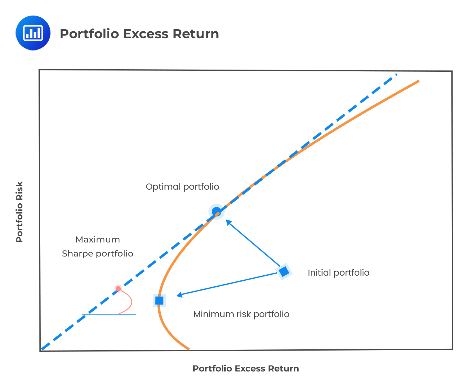 It reflects how the portfolio moves from the origin to the global minimum-risk portfolio. The efficient frontier is shown as a dashed line.
The ratio of all expected returns to the marginal VaRs must be equal. At the optimum point, this is represented by:
$$ \cfrac {{ \text{E} }_{ \text{i} }}{ \Delta{ \text{VaR} }_{ \text{i} }} = \cfrac {{ \text{E} }_{ \text{i} }}{{ \beta }_{ \text{i} }} $$
This ratio is a constant, and it is a restatement of the capital asset pricing model, saying that the portfolio needs to be mean-variance efficient. The expected return on a component must be proportional to the beta relative of this portfolio, given by:
$$ { \text{E} }_{ \text{i} }={ \text{E} }_{ \text{m} } { \beta }_{ \text{i} } $$
Practice Question
The portfolio of X&M Bank is comprised of two foreign currencies, the Euro (EUR) and Sterling Pound (GBP). Suppose that there is no correlation between these two currencies and that they have a 5% and 9% probability of default against the dollar, respectively. The portfolio has USD 2.1 million invested in the EUR and USD 1.9 million invested in the GBP. X&M is considering increasing the GBP position by USD 12,500.
Using the marginal VaR method, calculate the incremental VaR with the assumption that \(\alpha=1.65\).
- USD 1,578.75.
- USD 2,317.85.
- USD 1,432.65.
- USD 2,561.25.
The correct answer is A.
We determine the dollar volatility by calculating the product:
$$ \sum { x } =\begin{bmatrix} { 0.05 }^{ 2 } & 0 \\ 0 & { 0.09 }^{ 2 } \end{bmatrix}\begin{bmatrix} $2.1 \\ $1.9 \end{bmatrix}=\begin{bmatrix} { 0.05 }^{ 2 }\times $2.1+0\times $1.9 \\ 0\times $2.1+{ 0.09 }^{ 2 }\times $1.9 \end{bmatrix}=\begin{bmatrix} $0.00525 \\ $0.01539 \end{bmatrix} $$
Therefore, the portfolio variance in dollar returns is:
$$ { \sigma }_{ P }^{ 2 }{ W }^{ 2 }={ x }^{ \prime }\sum { x } =\begin{bmatrix} \begin{matrix} $2.1 & \quad $1.9 \end{matrix} \end{bmatrix}\begin{bmatrix} $0.00525 \\ $0.01539 \end{bmatrix}=$2.1\times 0.00525+$1.9\times 0.01539 $$
$$ =0.040266 $$
The dollar volatility of the portfolio is:
$$ \sqrt { 0.040266 } =$0.201\quad million $$
The marginal VaR is given as:
$$\Delta VaR=\alpha \frac { cov\left( R,{ R }_{ P } \right) }{ { \sigma }_{ P } } $$
Thus, the marginal VaR for the Euro position is as follows:
$$\Delta VaR=1.65\frac { $0.00525 }{ $0.201 } =$0.0431$$and the marginal VaR for the pound position is as follows:
$$\Delta VaR=1.65\frac { $0.01539 }{ $0.201 } =$0.1263$$Since the two positions are uncorrelated, the incremental VaR of an additional $12,500 investment in the pound position would simply be $12,500 times 0.1263, or $1,578.75.
Practice calculating diversified VaR, understand portfolio risk analytics, confidence intervals, and aggregation effects as used in FRM risk management frameworks.
Offered by AnalystPrep


Get Ahead on Your Study Prep This Cyber Monday! Save 35% on all CFA® and FRM® Unlimited Packages. Use code CYBERMONDAY at checkout. Offer ends Dec 1st.