


The Black-Scholes-Merton Model
After completing this reading you should be able to: Explain the lognormal property... Read More
After completing this reading, you should be able to:
The mean-variance framework uses the expected mean and standard deviation to measure the financial risk of portfolios. Under this framework, it is necessary to assume that returns follow a specified distribution, usually the normal distribution.
The normal distribution is particularly common because it concentrates most of the data around the mean return. 66.7% of returns occur within plus or minus one standard deviations of the mean. A whopping 95% of the returns occur within plus or minus two standard deviations of the mean.
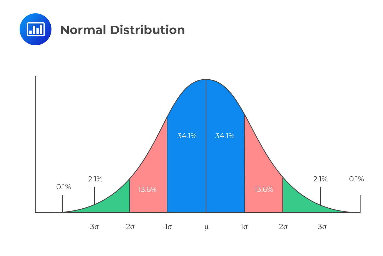 Investors are generally concerned with downside risk and are therefore interested in probabilities that lie to the left of the expected mean.
Note the expected return does not imply the anticipated return but rather the average returns. On the other hand, the risk is measured using the standard deviation of returns.
The expected returns for an asset with corresponding probabilities are given below:
$$ \begin{array}{c|c} \textbf{Return (%)} & \textbf{Probability} \\ \hline {10\%} & {0.25} \\ \hline {-20\%} & {0.09} \\ \hline {15\%} & {0.40} \\ \hline {7\%} & {0.06} \\ \hline {30\%} & {0.20} \end{array} $$
Calculate the expected return and standard deviation of the asset return.
To calculate the expected return, we weight the expected return by their corresponding probability. That is:
$$ \bar { \text{R} } =\sum _{ \text{i}=1 }^{ \text{n} }{ { \text{p} }_{ \text{i} }\text{R} } $$
So for this case,
$$ \begin{align*} \bar { \text{R} } &= \left(0.10\times0.25\right)+\left(-0.20\times0.09\right)+\left(0.15\times0.40\right)+\left(0.07\times0.06\right)+\left(0.30\times0.20\right) \\ &=0.1312=13.12\% \end{align*} $$
Recall that the variance for a variable X is given by:
$$ \text{Var}\left(\text{X}\right)=\text{E}\left({\text{X}}^{2}\right)-\left[\text{E}\left(\text{X}\right)\right]^{2} $$
Then the variance of the return R is given by:
$$ \text{Var}\left(\text{R}\right)=\text{E}\left({\text{R}}^{2}\right)-\left[\text{E}\left(\text{R}\right)\right]^{2} $$
The standard deviation is equal to the square root of the variance
$$ { \sigma }_{ \text{R} }=\sqrt{ \text{E} \left({ \text{R} }^{2}\right)-\left[ \text{E} \left({ \text{R} }\right) \right]^{2}} $$
Therefore,
$$ \begin{align*} \text{E} \left({ \text{R} }^{2}\right)=& \left({ 0.10 }^{ 2 }\times 0.25 \right)+ \left(\left( {-0.20} \right)^ {2} \times 0.09 \right)+\left( {0.15}^{2} \times {0.40} \right)+\left({0.07}^{2}\times{0.06}\right) \\ +&\left({0.30}^{2}\times{0.20}\right) \\ =&0.033394 \\ \Rightarrow { \sigma }_{ \text{R} }=&\sqrt{{0.033394}-\left[0.1312\right]^{2}}=0.1272=12.72\% \end{align*} $$
Consider two investments with respective means \({\mu}_{1}\) and \({\mu}_{2}\). Suppose that an investor wishes to invest in both investments with a proportion of \(\text{w}_{1}\) in the first investment and \(\text{w}_{2}\) in the second investment. It is safe to state that \(\text{w}_{2}=1-\text{w}_{1}\).
The portfolio expected return is equivalent to weighted returns from individual investments. That is:
$$ {\mu}_{\text{p}}=\text{w}_{1}{\mu}_{1} +\text{w}_{2}{\mu}_{2} $$
The variance of the portfolio expected return is given by:
$$ { \sigma }_{ \text{P} }^{ 2 }={ \text{w} }_{ 1 }^{ 2 }{ \sigma }_{ 1 }^{ 2 }+{ \text{w} }_{ 2 }^{ 2 }{ \sigma }_{ 2 }^{ 2 }+{ 2\rho \text{w} }_{ 1 }{ \text{w} }_{ 2 }{ \sigma }_{ 1 }{ \sigma }_{ 2 } $$
Where
\({\sigma}_1\): standard deviation of the first investment
\({\sigma}_2\): standard deviation of the second investment
\(\rho\): correlation between investment the first and the second investment
Therefore, the standard deviation of the portfolio is given by:
$$ { \sigma }_{ \text{P} }=\sqrt{{ \text{w} }_{ 1 }^{ 2 }{ \sigma }_{ 1 }^{ 2 }+{ \text{w} }_{ 2 }^{ 2 }{ \sigma }_{ 2 }^{ 2 }+{ 2\rho \text{w} }_{ 1 }{ \text{w} }_{ 2 }{ \sigma }} $$
Note that the variance of the portfolio can be written as:
$$ { \sigma }_{ \text{P} }^{ 2 }={ \text{w} }_{ 1 }^{ 2 }{ \sigma }_{ 1 }^{ 2 }+{ \text{w} }_{ 2 }^{ 2 }{ \sigma }_{ 2 }^{ 2 }+{ 2 \text{w} }_{ 1 }{ \text{w} }_{ 2 }\text{ Cov }\left({ \text{R} }_{1},{ \text{R} }_{2} \right) $$
This is true from the fact that:
$$ \begin{align*} \text{ Corr }\left({ \text{R} }_{1},{ \text{R} }_{2} \right)&={ \rho }=\cfrac{\text{ Cov }\left({ \text{R} }_{1},{ \text{R} }_{2} \right)}{{ \sigma }_{ 1 }{ \sigma }_{ 2 }} \\ \Rightarrow \text{ Cov }\left({ \text{R} }_{1},{ \text{R} }_{2} \right)&={ \rho }{ \sigma }_{ 1 }{ \sigma }_{ 2 } \end{align*} $$
An investor invests in two assets X and Y, with an expected return of 10% and 15%. The investor invests 45% of his funds in asset X and the rest in asset Y. The correlation coefficient is 0.45. Given that the standard deviation of asset X is 15% and Y is 30%, what are the expected return and standard deviations of the portfolio?
The portfolio expected return is given by:
$$ \begin{align*} { \mu }_{ \text{p} }&={ \text{w} }_{ \text{X} } { \mu }_{ \text{X} }+{ \text{w} }_{ \text{Y} } { \mu }_{ \text{Y} } \\ &=0.10\times0.45+0.15\times0.55 \\ &=0.1275=12.75\% \end{align*} $$
The portfolio standard deviation is given by:
$$ \begin{align*} { \sigma }_{ \text{P} }&=\sqrt{{ \text{w} }_{ 1 }^{ 2 }{ \sigma }_{ 1 }^{ 2 }+{ \text{w} }_{ 2 }^{ 2 }{ \sigma }_{ 2 }^{ 2 }+{ 2\rho \text{w} }_{ 1 }{ \text{w} }_{ 2 }{ \sigma }_{ 1 }{ \sigma }_{ 2 }} \\ &=\sqrt{ {0.45}^{2}\times{0.15}^{2}+{0.55}^{2}\times{0.3}^{2}+{2}\times{0.45}\times{0.45}\times{0.55}\times{0.15}\times{0.3} } \\ &=\sqrt{0.041805}=0.2325=23.25\% \end{align*} $$
Calculating the portfolio expected return and standard deviation can be extended to a portfolio with n investments. The portfolio expected return for n returns is given by:
$$ { \mu }_{ \text{p} } =\sum _{ \text{i}=1 }^{ \text{n} }{ { \text{w} }_{ \text{i} } { \mu }_{ \text{i} }} $$
Where \({\mu}_{\text{i}}\) and \({\text{w}}_{\text{i}}\) are the mean return and weight of ith investment
And then the standard deviation of the portfolio is given by:
$$ { \sigma }_{ \text{P} }=\sum _{ \text{i}=1 }^{ \text{n} }{ \sum _{ \text{j}=1 }^{ \text{n} }{ { \rho }_{ \text{ij} }{ \text{w} }_{ \text{i} }{ \text{w} }_{ \text{j} }{ \sigma }_{ \text{i} }{ \sigma }_{ \text{j} } } } $$
where \({ρ}_{\text{ij}}\) is the correlation coefficient between investments i and j. Other variables are intuitively definitive.
The efficient frontier represents the set of optimal portfolios that offers the highest expected return for a defined level of risk or the lowest risk for a given level of expected return. This concept can be represented on a graph by plotting the expected return (Y-axis) against the standard deviation (X-axis).
For every point on the efficient frontier, at least one portfolio can be constructed from all available investments with the expected risk and return corresponding to that point. Portfolios that do not lie on the efficient frontier are suboptimal: those that lie below the line do not provide enough return for the level of risk. Those that lie on the right of the line have a higher level of risk for the defined rate of return.
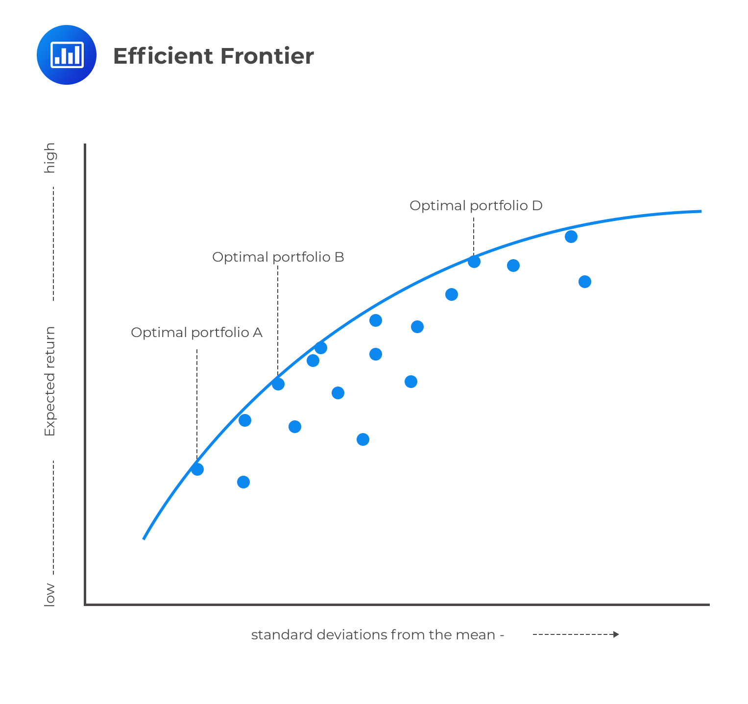 The choice between optimal portfolios A, B, and D above will depend on an individual investor’s appetite for risk. A very risk-averse investor will choose portfolio A because it offers an optimal return at the lowest risk, whereas an investor with room for more risk might pick D. After all, it offers the highest optimal return at the highest risk.
Note that, the efficient frontier above considers only the risky assets. Now, consider when we introduce a risk-free investment with a return of \({\text{R}}_{\text{F}}\). It can be shown that the efficient frontier is a straight line. That is, there is a linear relationship between the expected return and the standard deviation of return.
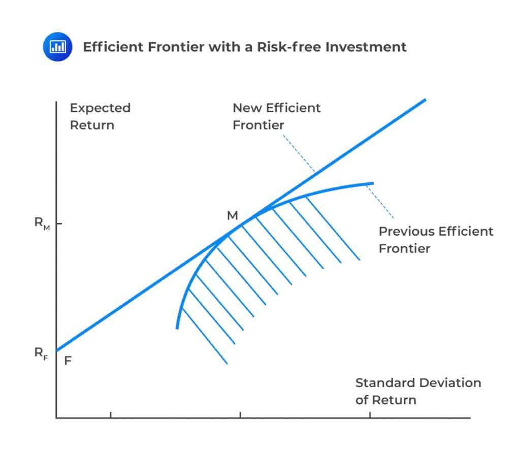 F represents the risk-free return on the diagram above. Note that risk-free asset sits on the efficient frontier because you cannot get a higher return with no risk, and you cannot have less risk than zero. Consider the tangent line FM. By proportioning our investment between the risk-free asset F and the risky asset M (market portfolio), we can obtain a risk-return that lies on the line FM combination. In other words, the risk-return tradeoff is a linear function.
Denote the risk-free return by \({\text{R}}_{\text{F}}\) (with a standard deviation of 0). Also, let the market portfolio return be \({\text{R}}_{\text{M}}\), and its standard deviation is \({\sigma}_{\text{M}}\). Let the proportion of funds in a risky portfolio be \(\beta\) and that in risk-free assets, be \(1-{\beta}\). Now using the formula
$$ { \mu }_{ \text{p} }={ \text{w} }_{ 1 } { \mu }_{ 1 }+{ \text{w} }_{ 2 } { \mu }_{ 2 } $$
We have \({ \text{w} }_{ 1 }=1-{ \beta }, { \text{w} }_{ 2 }={ \beta }, { \mu }_{ 1 }={ \text{R} }_{ \text{F} }, { \mu }_{ 2 }={ \text{R} }_{ \text{M} } \) so that return from the portfolio is given by
$$ \begin{align*} { \mu }_{ \text{p} }&={ \text{R} }_{ \text{F} } \left(1-{ \beta }\right)+ \beta{ \text{R} }_{ \text{M} } \\ \Rightarrow \beta&= \cfrac{{ \mu }_{ \text{p} }-{ \text{R} }_{ \text{F} }}{{ \text{R} }_{ \text{M} }-{ \text{R} }_{ \text{F} }} \end{align*} $$
Also, the standard deviation of a portfolio with two components is given by
$$ { \sigma }=\sqrt{{ \text{w} }_{ 1 }^{ 2 }{ \sigma }_{ \text{F} }^{ 2 }+{ \text{w} }_{ 2 }^{ 2 }{ \sigma }_{ \text{M} }^{ 2 }+{ 2\rho \text{w} }_{ 1 }{ \text{w} }_{ 2 }{ \sigma }_{ \text{F} }{ \sigma }_{ \text{M} }} \\ $$
But \({ \sigma }_{ \text{F} }=0\)
$$ \Rightarrow { \sigma }=\sqrt{{0}+{ \text{w} }_{2}^{2} { \sigma }_{ \text{M} }^{2}+{0}}={ \text{w} }_{2} { \sigma }_{ \text{M} }={ \beta }{ \sigma }_{ \text{M} } $$
Therefore,
$$ \begin{align*} { \sigma }&={ \sigma }_{ \text{M} } \left( \cfrac{ { \mu }_{ \text{P} }-{ \text{R} }_{ \text{F} }}{{ \text{R} }_{ \text{M} }-{ \text{R} }_{ \text{F} }} \right) \\ \Rightarrow{ \sigma }&={ \mu }_{ \text{p} }\left( \cfrac{ { \sigma }_{ \text{M} } }{{ \text{R} }_{ \text{M} }-{ \text{R} }_{ \text{F} }} \right)-\cfrac{ { \sigma }_{ \text{M} }{ \text{R} }_{ \text{F} } }{{ \text{R} }_{ \text{M} }-{ \text{R} }_{ \text{F} }} \end{align*} $$
The efficient frontier involving a risk-free asset also shows that the investor should invest in risky assets (in this case, M) by borrowing and lending at a risk-free rate \({\text{r}}_{\text{F}}\). For instance, we assume that an investor borrows at the rate \({\text{r}}_{\text{F}}\) so that now we are considering the efficient frontier beyond M. If this is the case, then \({\beta}>{1}\) and the proportion of amount borrowed will be \({\beta}-{1}\), and the total amount available is \(\beta\) multiplied by available funds. Assume now that we invest in risky asset M. Then the expected return is:
$$ \beta{ \text{r} }_{ \text{M} }-\left({ \beta }-1\right) { \text{R} }_{ \text{F} }=\left(1-{\beta}\right) { \text{r} }_{ \text{F} }+\beta{ \text{r} }_{ \text{M} } $$
The standard deviation can be shown to be \({\beta}{\sigma}_{\text{M}}\), which is similar to arguments for the points below point M.
Therefore, it is safe to say risk-averse investors will invest in points on line FM and close to F, and those investors that are risk-seeking will invest on points close to M or even points beyond M on line FM.
The normal distribution, also called Gaussian distribution, is a widely used continuous distribution with two parameters: mean denoted by \({ \mu }\) and the standard deviation denoted by \({ \sigma }\). The density function of the normal distribution is given by
$$ \text{f}\left( \text{x} \right) =\cfrac { 1 }{ \sqrt { 2\pi { \sigma }^{ 2 } } } { \text{e} }^{ -\cfrac { { \left( \text{x}-\mu \right) }^{ 2 } }{ 2{ \sigma }^{ 2 } } } $$
The shape of the standard curve is as shown below.
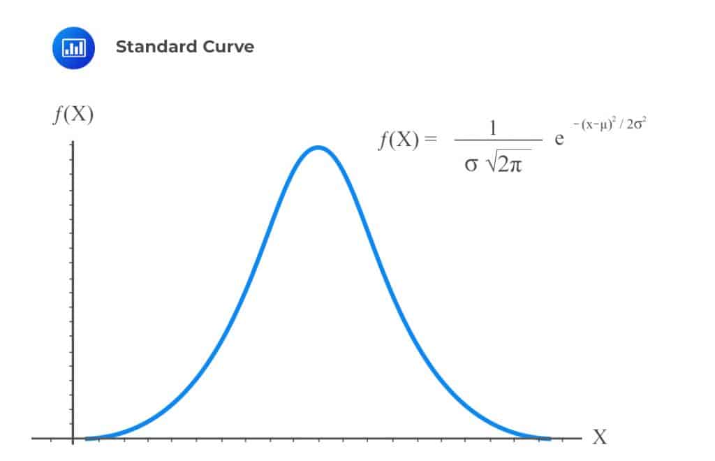 The height of the normal distribution is equivalent to the probability that a value X has occurred. This is commonly stated as \({\text{X}}\sim {\text{N}}({\mu},{\sigma}^{2} )\). Values close to the center of the distribution are most likely to occur while those values at the tails of the distribution are less likely to occur.
Note that, similar to other probability distributions, the probability that a value lies between \(a\) and \(b\) is equivalent to the area under the curve between \(a\) and \(b\). This can be thought of as the cumulative distribution up to a point \(b\) less the cumulative distribution up to point \(a\).
A standard normal distribution has a mean of 0 and a standard deviation of 1. In other words, \({ \mu }\)=0 and \({ \sigma }\)=1. As such, the normal distribution density function reduces to:
$$ \text{f}\left( \text{x} \right) =\cfrac { 1 }{ \sqrt { 2\pi } } { \text{e} }^{ -\cfrac { { \text{x} }^{ 2 } }{ 2} } $$
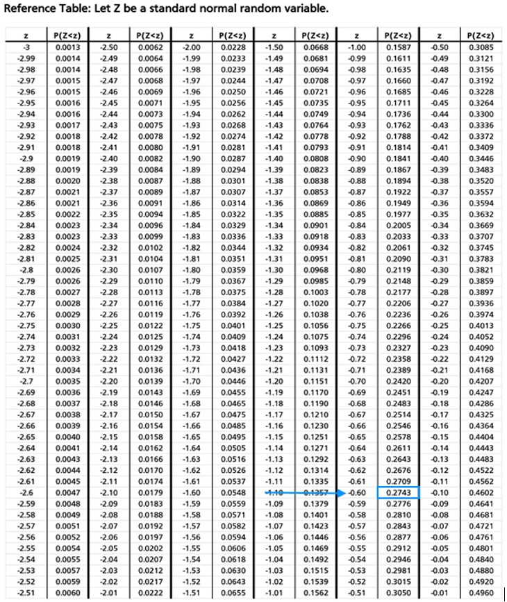
The normal tables give a cumulative distribution of the standard normal distribution. For normal distribution with the mean \({ \mu }\) and the standard deviation \({ \sigma }\), it can be transformed into z-scores, which gives cumulative probability up to a value x for standard normal. The z-score is defined by:
$$ \text{z}=\cfrac{\text{x}-{\mu}}{\sigma} $$
Where \(\text{z}{ \sim }\text{N}\)(0,1).
For example, consider a normal distribution with a mean of 4 and a standard deviation of 5. What is the probability that a value X is less than 7? Using standard normal transformation,
$$ \begin{align*} \text{Pr}({ X }<{7})& = {Pr}( \cfrac { { { X } }-{ \mu } }{ \sigma } < \cfrac { { 7-4 } }{ 5 } ) = 0.6\\ &=Pr(z<0.6)=Φ(0.6)=1-0.2743=0.7257 \end{align*} $$
Note that the standard normal table is usually provided in exam.
In this case, the table provided is of negative z-values; as such, if we want to read the probability of \(P(z<0.6)\) then we will be forced to use \(1-P(z<-0.6)\) since the table gives probabilities for negative z-values yet, we want the probability for a positive z-value.
A normal distribution is usually assumed to apply to financial data because financial analysts are mostly concerned with the mean and standard deviation. However, financial variables have fatter tails than the normal distribution. A large number of portfolio returns also tend to have fatter tails than the normal distribution. For instance, the means created can have fatter tails. Consider the diagram below.
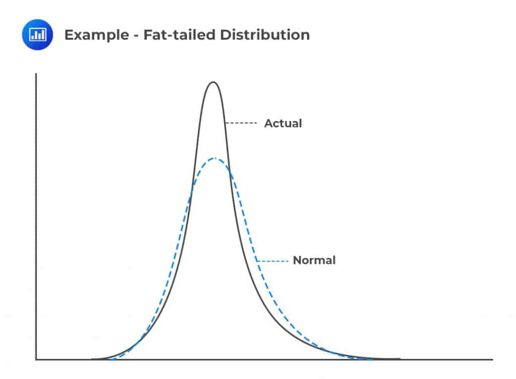 The diagram shows that the normal distribution and the actual distribution have equal standard deviations, but the actual distribution is more peaked and has fatter tails than the normal distribution. In other words, the actual distribution suggests that small and large changes frequently occur while intermediate events occur less frequently.
As discussed earlier in this chapter, we have seen that assuming a normal distribution for financial variables (by use of mean and standard deviation) may underestimate the probability of the adverse events.
The standard deviation can be a perfect measure of risk, but it does not capture the tails of the probability distribution.
VaR is a risk measure that is concerned with the occurrence of adverse events and their corresponding probability. VaR is built from two parameters: the time horizon and the confidence level. Therefore, we can say that VaR is the loss that we do not anticipate to be exceeded over a given time period at a specified confidence level.
For example, consider a time horizon of 30 days and a confidence interval of 98%. Therefore 98% VaR of USD 5 million implies that we are 98% confident that over the next 30 days, the loss will be less than USD 5 million. Similarly, we can say that we are 2% confident that over the next 30 days, the loss will be greater than USD 5 million.
Consider the following loss distribution density function curve:
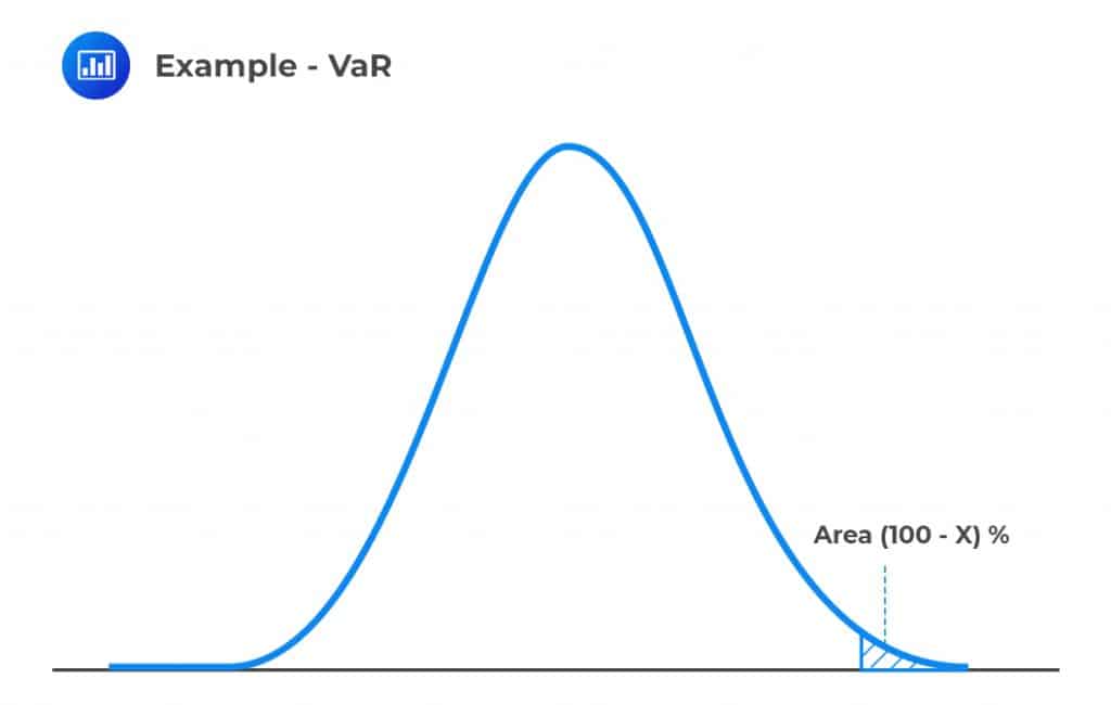 Therefore, calculating X% VaR involves finding the loss that has an X% chance of being exceeded, or the area under the curve that equal to (100-X)%.
Consider the following examples:
The investment return over a period of time has a normal loss distribution with a mean of -200 and a variance of 300. What is 99% VaR of the loss distribution?
Denote the VaR level by t, then we need:
$$ \text{P}\left({ \text{X} }<{ \text{t} }\right)=0.99 $$
(Note we can also use \(\text{P}({\text{X}}>{\text{t}})\)=0.01)
Standardizing the normal distribution with a given mean and standard deviation, we have:
$$ \begin{align*} \text{P}\left( \text{z}<\cfrac { \text{t}-(-200)}{ \sqrt{300} } \right) &=0.99 \\ \Rightarrow \Phi \left( \cfrac { \text{t}+200 }{ \sqrt{300} } \right) &=\left( 0.99 \right) \\ \Rightarrow \cfrac { \text{t}+200 }{ \sqrt{300}} &={ \Phi }^{ -1 }\left( 0.99 \right) \end{align*}$$
Now, \({\Phi}^{-1}\)(0.99) is the inverse of standard normal cumulative probability. To do this using a standard table, look for 0.99 (or closest value) in the table and read the corresponding vertical and horizontal values and add them. In other words, we are reversing the reading of the standard normal table.
In our cases, consider the following table:
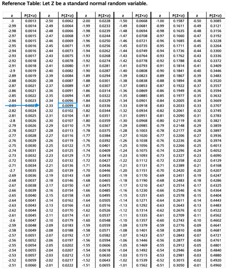
And thus:
$$ \begin{align*} { \Phi }^{ -1 }\left( 0.99 \right) &=2.33\\ \therefore \cfrac { \text{t}+200 }{ \sqrt{300} } &=2.33\\ \Rightarrow \text{t}&=-200+\sqrt{300}\times 2.33=-159.64 \end{align*} $$
The VaR level is -159.64 at a 99% confidence level.
The loss distribution of investment is as shown below:
$$ \begin{array}{c|c} \textbf{Amount of Loss} & \textbf{Probability} \\ \hline \text{USD 10 Million} & {75\%} \\ \hline \text{USD 13 Million} & {22\%} \\ \hline \text{US 17 million} & {3\%} \end{array} $$
What is the value of the 99% VaR?
To find the 99%, we need to find the cumulative probability distribution and locate 99%:
$$ \begin{array}{c|c|c} \textbf{Amount of Loss} & \textbf{Probability} & \textbf{Cumulative Probability Range} \\ \hline \text{USD 10 Million} & {75\%} & \text{0 to 75%} \\ \hline \text{USD 13 Million} & {22\%} & \text{75% to 97%} \\ \hline \text{US 17 million} & {3\%} & \text{97% to 100%} \end{array} $$
Therefore, with a confidence level of 99%, the VaR value is USD 17 million because 99% falls the range of 97% and 100% (the last range).
Note that if we reduce our confidence level to 95%, VaR will change to USD 13 million because 95% falls between 75% to 97% cumulative probability range.
However, if the confidence level is 97%, then we could have two VaR values: USD 13 million and USD 17 million. This will be ambiguous, and so the best estimate is the average of the values, which is USD 15 million.
Recall the VaR does not describe the worst possible loss. For instance, if 99% VaR is USD 10 million, we know that we are 1% certain that the loss will exceed USD 10 million. From the VaR level, we cannot say that the loss is greater than 20 million or USD 50 million. Therefore, VaR sets a risk measure equal to a certain percentile of the loss distribution and does not consider the possible losses beyond the VaR level.
Expected shortfall (ES) is a risk measure that considers the expected losses beyond the VaR level. In other words, ES is the expected loss conditional that the loss is greater than the VaR level.
Exam tip: Expected shortfall is also called conditional value at risk (CVaR), average value at risk (AVaR), or expected tail loss (ETL). Think about this as the average loss beyond the VaR.
When the losses are normally distributed with the mean μ and standard deviation σ, then the ES is given by:
$$ \text{ES}=\mu +\sigma \left( \cfrac { { \text{e} }^{ -\cfrac { { \text{U} }^{ 2 } }{ 2 } } }{ \left( 1-{ \text{X} } \right) \sqrt { 2\pi } } \right) $$
Where
X = the confidence level; and
U = the point in the standard normal distribution that has a probability of X% of being exceeded.
The investment return over a period of time has a normal loss distribution with a mean of -200 and a standard deviation of 300. What is 99% Expected of the loss distribution?
We know that:
$$ \text{ES}=\mu +\sigma \left( \cfrac { { \text{e} }^{ -\frac { { \text{U} }^{ 2 } }{ 2 } } }{ \left( 1-{ \text{X} } \right) \sqrt { 2\pi } } \right) $$
Now, U=2.33
$$ \text{ES}={ -200 } + { 300 } \left( \cfrac { \text{e}^{ -\frac { { \left(2.33\right) }^{ 2 } }{ 2 } } }{ \left( 1-0.99 \right) \sqrt { 2\pi } } \right) =592.79$$
ES should always be greater than the VaR level because the ES gives us the average of the values that are in the tail exceeding VaR.
The loss distribution of investment is as shown below:
$$ \begin{array}{c|c} \textbf{Amount of Loss} & \textbf{Probability} \\ \hline \text{USD 20 Million} & {2\%} \\ \hline \text{USD 17 Million} & {8\%} \\ \hline \text{US 13 million} & {12\%} \\ \hline \text{US 10 million} & {78\%} \end{array} $$
What is the 95% expected shortfall (ES)?
At a 95% confidence level, we need to answer the question, “given that we are at 5% of the loss distribution, what is the value of the expected loss?”.Now looking at the probability column, it is clear to see that 5% tail distribution consists of a 2% probability that the loss is USD 20 million and 3% that the loss is USD 17 million. Conditioned that we are dealing with tail distribution, then there is a 2/5 chance that the loss is USD 20 million and a 3/5 chance that the loss is USD 17 million. Therefore, the expected shortfall is given by:
$$ \cfrac{2}{5}\times20+\cfrac{3}{5}\times17=18.20 $$
Again, note that the 97% VaR is USD 10 million, which is less than ES.
A risk measure summarizes the entire distribution of dollar returns X by one number, \({ \rho }\)(X). There are four desirable properties every risk measure should possess. These are:
Interpretation: If a portfolio has systematically lower values than another, it must have a greater risk in each state of the world. In other words, if a portfolio gives undesirables results than the others, then it must be riskier.
Interpretation: When two portfolios are combined, their total risk should be less than (or equal to) the sum of their risks. Merging of portfolios ought to reduce risk. This property captures the implications of diversification. If two portfolios are perfectly correlated, then the overall risk is the sum of their risk when considered separately. However, if the two portfolios are not perfectly correlated, their overall risk should decrease due to diversification benefits.
Interpretation: Increasing the size of a portfolio by a factor k should result in a proportionate scale in its risk measure. For instance, if we increase the portfolio size by a quarter, then the risk should be increased by a quarter.
Interpretation: Adding cash h to a portfolio should reduce its risk by h. Like X, h is measured in dollars. This property reflects that more cash acts as a “loss absorber” and can be taken as a replacement for capital.
If a risk measure satisfies all four properties, then it is a coherent risk measure. Expected shortfall is a coherent risk, but VaR is not.
Value at risk is not a coherent risk measure because it fails the subadditivity test. Here’s an illustration:
Suppose we want to calculate the VaR of a portfolio at 95% confidence over the next year of two zero-coupon bonds (A and B) scheduled to mature in one year. Assume that:
Given these conditions, the 95% VaR for holding either of the bonds is 0 because the probability of default is less than 5%. Now, what is the probability ‘P’ that at least one bond defaults?
$$ \text{P}=0.04\times0.96+0.96\times0.04+0.04\times0.04=7.84 $$
The probability of at least one default is 7.84%, which exceeds 5%.
So if we held a portfolio that consisted of 50% A and 50% B, then the 95% VaR = 0.7 × 0.5 + 0 × 0.5 = 35%
This violates the subadditivity principle, and VaR is, therefore, not a coherent risk measure.
Practice Question
Ann Conway, FRM, has spent the last several months trying to develop a new risk measure to appraise a set of defaultable zero-coupon bonds owned by her employer. Prior to its use, her supervisor has asked her to demonstrate that it is a coherent risk measure. The results are listed below:
Given:
- X and y are state-contingent payoffs of two different bond portfolios.
- \(\text{P}\left(\text{x}\right) \text{ and } \text{P}\left(\text{y}\right) \)are risk measures for portfolio x and portfolio y.
- K and l are arbitrary constants, with \(\text{k}>0\)
Which of the following equations shows that Conway’s risk measure is not coherent?
- \(\text{P}\left(\text{kx}\right)=\text{kP}\left(\text{x}\right)\)
- \(\text{P}\left(\text{x}\right)+\text{P}\left(\text{y}\right)≥\text{P}\left(\text{x+y}\right)\)
- \(\text{P}\left(\text{x}\right)≤\text{P}\left(\text{y}\right) \text{ if } {\text x} \le {\text y}\)
- \(\text{P}\left(\text{x+l}\right)=\text{P}\left(\text{x}\right)−\text{l}\)
The correct answer is C.
Option C, as represented above, shows that the risk measure does not satisfy the monotonicity property. Monotonicity requires that \( \text{P}\left(\text{x}\right)≥\text{P}\left(\text{y}\right) \text{ if } \text{x}≤\text{y}.\) (If a portfolio has systematically lower values than another, in each state of the world, it must have a greater risk.)
Option A demonstrates that the measure satisfies the homogeneity property.
Option B demonstrates that the measure satisfies the subadditivity property.
Option D demonstrates that the measure satisfies the translation invariance property.
Access FRM practice questions, study notes, mock exams, and video lessons with AnalystPrep.
Offered by AnalystPrep


Get Ahead on Your Study Prep This Cyber Monday! Save 35% on all CFA® and FRM® Unlimited Packages. Use code CYBERMONDAY at checkout. Offer ends Dec 1st.