


Modeling and Hedging Non-Parallel Term ...
After completing this reading you should be able to: Describe principal components analysis... Read More
After completing this reading you should be able to:
This section is about the calculation of the standard error, hypotheses testing, and confidence interval construction for a single regression in a multiple regression equation.
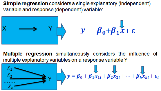
In a previous chapter, we looked at simple linear regression where we deal with just one regressor (independent variable). The response (dependent variable) is assumed to be affected by just one independent variable.
Multiple regression, on the other hand, simultaneously considers the influence of multiple explanatory variables on a response variable Y. We may want to establish the confidence interval of one of the independent variables. We may want to evaluate whether any particular independent variable has a significant effect on the dependent variable. Finally, We may also want to establish whether the independent variables as a group have a significant effect on the dependent variable. In this chapter, we delve into ways all this can be achieved.
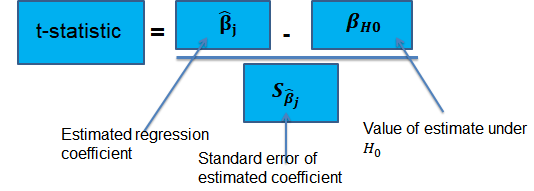
Suppose that we are testing the hypothesis that the true coefficient \({ \beta }_{ j }\) on the \(j\)th regressor takes on some specific value \({ \beta }_{ j,0 }\). Let the alternative hypothesis be two-sided. Therefore, the following is the mathematical expression of the two hypotheses:
$$ { H }_{ 0 }:{ \beta }_{ j }={ \beta }_{ j,0 }\quad vs.\quad { H }_{ 1 }:{ \beta }_{ j }\neq { \beta }_{ j,0 } $$
This expression represents the two-sided alternative. The following are the steps to follow while testing the null hypothesis:
$$ p-value=2\Phi \left( -|{ t }^{ act }| \right) $$
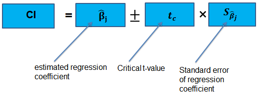
The confidence interval for a regression coefficient in multiple regression is calculated and interpreted the same way as it is in simple linear regression.
The t-statistic has n – k – 1 degrees of freedom where k = number of independents
Supposing that an interval contains the true value of \({ \beta }_{ j }\) with a probability of 95%. This is simply the 95% two-sided confidence interval for \({ \beta }_{ j }\). The implication here is that the true value of \({ \beta }_{ j }\) is contained in 95% of all possible randomly drawn variables.
Alternatively, the 95% two-sided confidence interval for \({ \beta }_{ j }\) is the set of values that are impossible to reject when a two-sided hypothesis test of 5% is applied. Therefore, with a large sample size:
$$ 95\%\quad confidence\quad interval\quad for\quad { \beta }_{ j }=\left[ { \hat { \beta } }_{ j }-1.96SE\left( { \hat { \beta } }_{ j } \right) ,{ \hat { \beta } }_{ j }+1.96SE\left( { \hat { \beta } }_{ j } \right) \right] $$
In this section, we consider the formulation of the joint hypotheses on multiple regression coefficients. We will further study the application of an \(F\)-statistic in their testing.
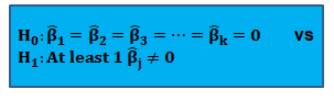
In multiple regression, we cannot test the null hypothesis that all slope coefficients are equal 0 based on t-tests that each individual slope coefficient equals 0. Why? individual t-tests do not account for the effects of interactions among the independent variables.
For this reason, we conduct the F-test which uses the F-statistic. The F-test tests the null hypothesis that all of the slope coefficients in the multiple regression model are jointly equal to 0, .i.e.,
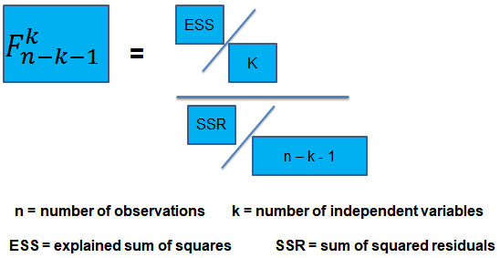
The F-statistic, which is always a one-tailed test, is calculated as:
To determine whether at least one of the coefficients is statistically significant, the calculated F-statistic is compared with the one-tailed critical F-value, at the appropriate level of significance.
Decision rule:

Rejection of the null hypothesis at a stated level of significance indicates that at least one of the coefficients is significantly different than zero, i.e, at least one of the independent variables in the regression model makes a significant contribution to the dependent variable.
An analyst runs a regression of monthly value-stock returns on four independent variables over 48 months.
The total sum of squares for the regression is 360, and the sum of squared errors is 120.
Test the null hypothesis at the 5% significance level (95% confidence) that all the four independent variables are equal to zero.
\({ H }_{ 0 }:{ \beta }_{ 1 }=0,{ \beta }_{ 2 }=0,\dots ,{ \beta }_{ 4 }=0 \)
Versus
\({ H }_{ 1 }:{ \beta }_{ j }\neq 0\) (at least one j is not equal to zero, j=1,2… k )
ESS = TSS – SSR = 360 – 120 = 240
The calculated test statistic = (ESS/k)/(SSR/(n-k-1))
=(240/4)/(120/43) = 21.5
\({ F }_{ 43 }^{ 4 }\) is approximately 2.44 at 5% significance level.
Decision: Reject H0.
Conclusion: at least one of the 4 independents is significantly different than zero.
This is the bias in the OLS estimator arising when at least one included regressor gets collaborated with an omitted variable. The following conditions must be satisfied for an omitted variable bias to occur:
To determine the accuracy within which the OLS regression line fits the data, we apply the coefficient of determination and the regression’s standard error.
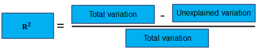
The coefficient of determination, represented by \({ R }^{ 2 }\), is a measure of the “goodness of fit” of the regression. It is interpreted as the percentage of variation in the dependent variable explained by the independent variables
\({ R }^{ 2 }\) is not a reliable indicator of the explanatory power of a multiple regression model.Why? \({ R }^{ 2 }\) almost always increases as new independent variables are added to the model, even if the marginal contribution of the new variable is not statistically significant. Thus, a high \({ R }^{ 2 }\) may reflect the impact of a large set of independents rather than how well the set explains the dependent.This problem is solved by the use of the adjusted \({ R }^{ 2 }\) (extensively covered in chapter 8)
The following are the factors to watch out when guarding against applying the \({ R }^{ 2 }\) or the \({ \bar { R } }^{ 2 }\):
Question 1
An economist tests the hypothesis that GDP growth in a certain country can be explained by interest rates and inflation.
Using some 30 observations, the analyst formulates the following regression equation:
$$ GDP growth = { \hat { \beta } }_{ 0 } + { \hat { \beta } }_{ 1 } Interest+ { \hat { \beta } }_{ 2 } Inflation $$
Regression estimates are as follows:
|
Coefficient |
Standard error |
|
|
Intercept |
0.10 |
0.5% |
|
Interest rates |
0.20 |
0.05 |
|
Inflation |
0.15 |
0.03 |
Is the coefficient for interest rates significant at 5%?
The correct answer is C.
We have GDP growth = 0.10 + 0.20(Int) + 0.15(Inf)
Hypothesis:
$$ { H }_{ 0 }:{ \hat { \beta } }_{ 1 } = 0 \quad vs \quad { H }_{ 1 }:{ \hat { \beta } }_{ 1 }≠0 $$
The test statistic is:
$$ t = \left( \frac { 0.20 – 0 }{ 0.05 } \right) = 4 $$
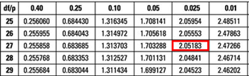
The critical value is t(α/2, n-k-1) = t0.025,27 = 2.052 (which can be found on the t-table).
 Decision: Since test statistic > t-critical, we reject H0.
Conclusion: The interest rate coefficient is significant at the 5% level.
Offered by AnalystPrep


