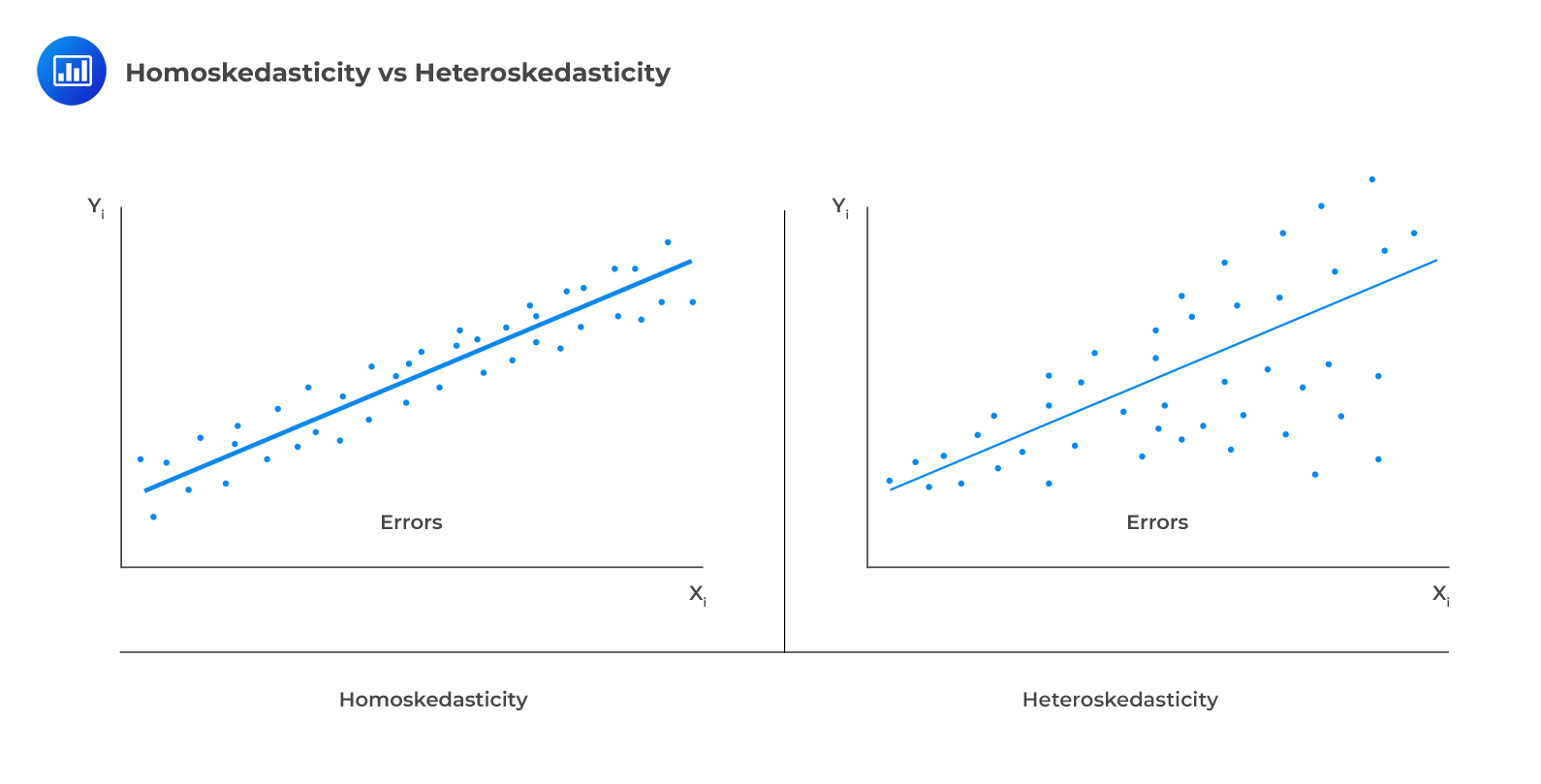
One of the assumptions underpinning multiple regression is that regression errors are homoscedastic. In other words, the variance of the error terms is equal for all observations:

$$E(\epsilon_{i}^{2})=\sigma_{\epsilon}^{2}, i=1,2,…,n$$

In reality, the variance of errors differs across observations. This is known as heteroskedasticity.

The following figure illustrates homoscedasticity and heteroskedasticity.

Types of Heteroskedasticity

Unconditional Heteroskedasticity

Unconditional heteroskedasticity occurs when the heteroskedasticity is uncorrelated with the values of the independent variables. Although this is a violation of the homoscedasticity assumption, it does not present major problems to statistical inference.

Conditional Heteroskedasticity

Conditional heteroskedasticity occurs when the error variance is related/conditional on the values of the independent variables. It poses significant problems for statistical inference. Fortunately, many statistical software packages can diagnose and correct this error.

Effects of Heteroskedasticity

     i. It does not affect the consistency of the regression parameter estimators.

     ii. Heteroskedastic errors make the F-test overall significance of the regression unreliable.

    iii. Heteroskedasticity introduces bias into estimators of the standard error of regression coefficients making the t-tests for the significance of individual regression coefficients unreliable.

   iv. More specifically, it results in inflated t-statistics and underestimated standard errors.

Testing Heteroskedasticity

Breusch-Pagan chi-square test

The Breusch-Pagan chi-square test looks at the regression of the squared residuals from the estimated regression equation on the independent variables. The presence of conditional heteroskedasticity in the original regression equation substantially explains the variation in the squared residuals.

The test statistic is given by:

$$\text{BP chi}-\text{square test statistic}=n\times{R^{2}}$$

Where:

• \(n\) = number of observations.
• \(R^{2}\) = the \(R^{2}\) in the regression of the squared residuals.

This test statistic is a chi-square random variable with k degrees of freedom.

The null hypothesis is that there is no conditional heteroskedasticity, i.e., the squared error term is uncorrelated with the independent variables. The Breusch-pagan test is a one-tailed test as we should be mainly concerned with heteroskedasticity for large values of the test statistic.

Example: Breusch-Pagan chi-square test

Consider the multiple regression of the price of the USDX on the inflation rates and the real interest rates. The investor regresses the squared residuals from the original regression on the independent variables. The new \(R^{2}\) is 0.1874. Test for the presence of heteroskedasticity at the 5% significance level.

Solution

The test statistic is:

$$\text{BP chi}- \text{square test statistic}=n\times{R^{2}}$$

$$\text{Test statistic}= 10\times0.1874=1.874$$

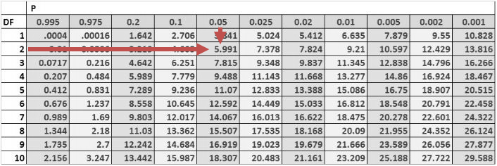
The one-tailed critical value for a chi-square distribution with two degrees of freedom at the 5% significance level is 5.991.

Therefore, we cannot reject the null hypothesis of no conditional heteroskedasticity. As a result, we conclude that the error term is NOT conditionally heteroskedastic.

Correcting Heteroskedasticity

In the investment world, it is crucial to correct heteroskedasticity as it may change inferences about a particular hypothesis test, thus impacting an investment decision. There are two methods that can be applied to correct heteroskedasticity:

1. Calculating robust standard errors: This approach corrects the standard errors of the model’s estimated coefficients to account for the conditional heteroskedasticity. These are also known as white-corrected standard errors. These standard errors are then used to calculate the t-statistics again using the original regression coefficients.
2. Generalized least squares: The original regression equation is modified to eliminate heteroskedasticity. The modified equation is then estimated, assuming that heteroskedasticity is no longer a problem.

Serial Correlation (Autocorrelation)

Autocorrelation occurs when the assumption that regression errors are uncorrelated across all observations is violated. In other words, autocorrelation is evident when errors in one period are correlated with errors in other periods. This is common with time-series data (which we will see in the next reading).

Types of Serial Correlation

Positive serial correlation

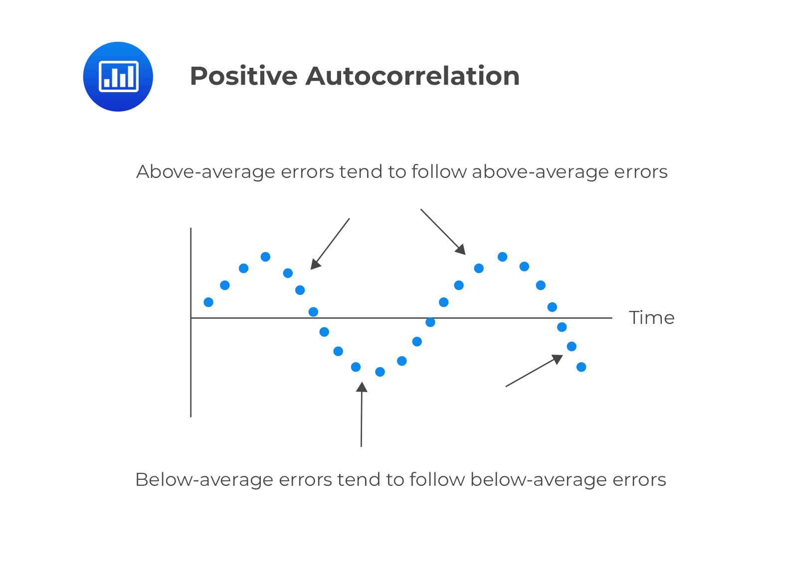
This is a serial correlation in which positive regression errors for one observation increases the possibility of observing a positive regression error for another observation.

Negative serial correlation

This is serial correlation in which a positive regression error for one observation increases the likelihood of observing a negative regression error for another observation.

Effects of Serial Correlation

Autocorrelation does not cause bias in the coefficient estimates of the regression. However, a positive serial correlation inflates the F-statistic to test for the overall significance of the regression as the mean squared error (MSE) will tend to underestimate the population error variance. This increases Type I errors (the rejection of the null hypothesis when it is actually true).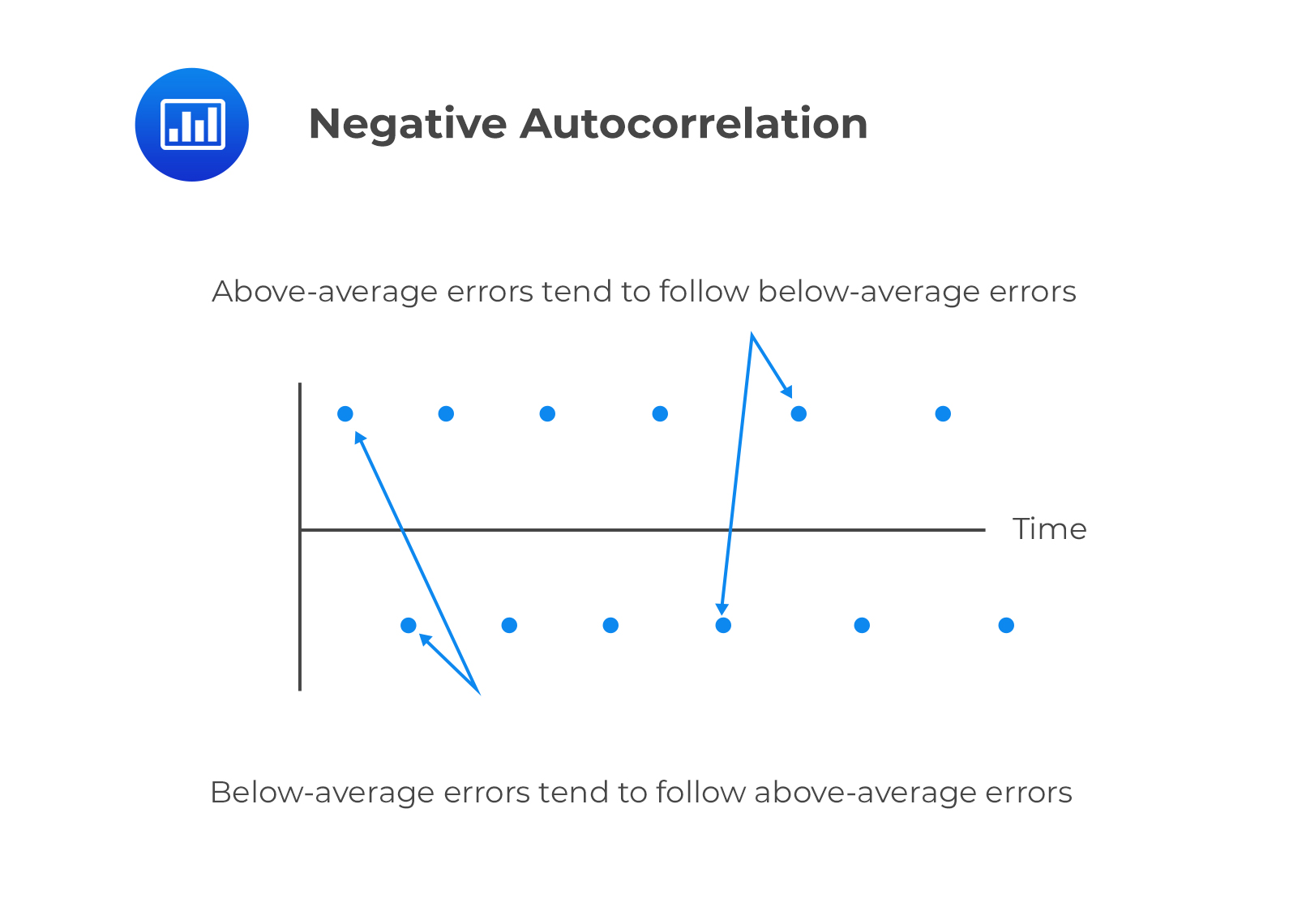

The positive serial correlation makes the ordinary least squares standard errors for the regression coefficients underestimate the true standard errors. Moreover, it leads to small standard errors of the regression coefficient, making the estimated t-statistics seem to be statistically significant relative to their actual significance.

On the other hand, negative serial correlation overestimates standard errors and understates the F-statistics. This increases Type II errors (The acceptance of the null hypothesis when it is actually false).

Testing for Serial Correlation

The first step of testing for serial correlation is by plotting the residuals against time. The other most common formal test is the Durbin-Watson test.

Durbin-Watson Test

The Durbin Watson tests the null hypothesis of no serial correlation against the alternative hypothesis of positive or negative serial correlation.

The Durbin-Watson Statistic (DW) is approximated by:

$$DW=2(1-r)$$

Where:

• \(r\) = Sample correlation between regression residuals from one period and the previous period.

The Durbin Watson statistic can take on values ranging from 0 to 4. i.e., \(0<DW<4\).

    i.  If there is no autocorrelation, the regression errors will be uncorrelated, and thus DW = 2.

$$DW=2(1-r)=2(1-0)=2$$

   ii. For positive serial autocorrelation, \(DW<2\).

 For example, if serial correlation of the regression residuals \(=1,DW=2(1-1)=0\)

   iii. For negative autocorrelation, \(DW>2\).

For example, if serial correlation of the regression regression residual \(=-1, DW=2(1-(-1))=4\).

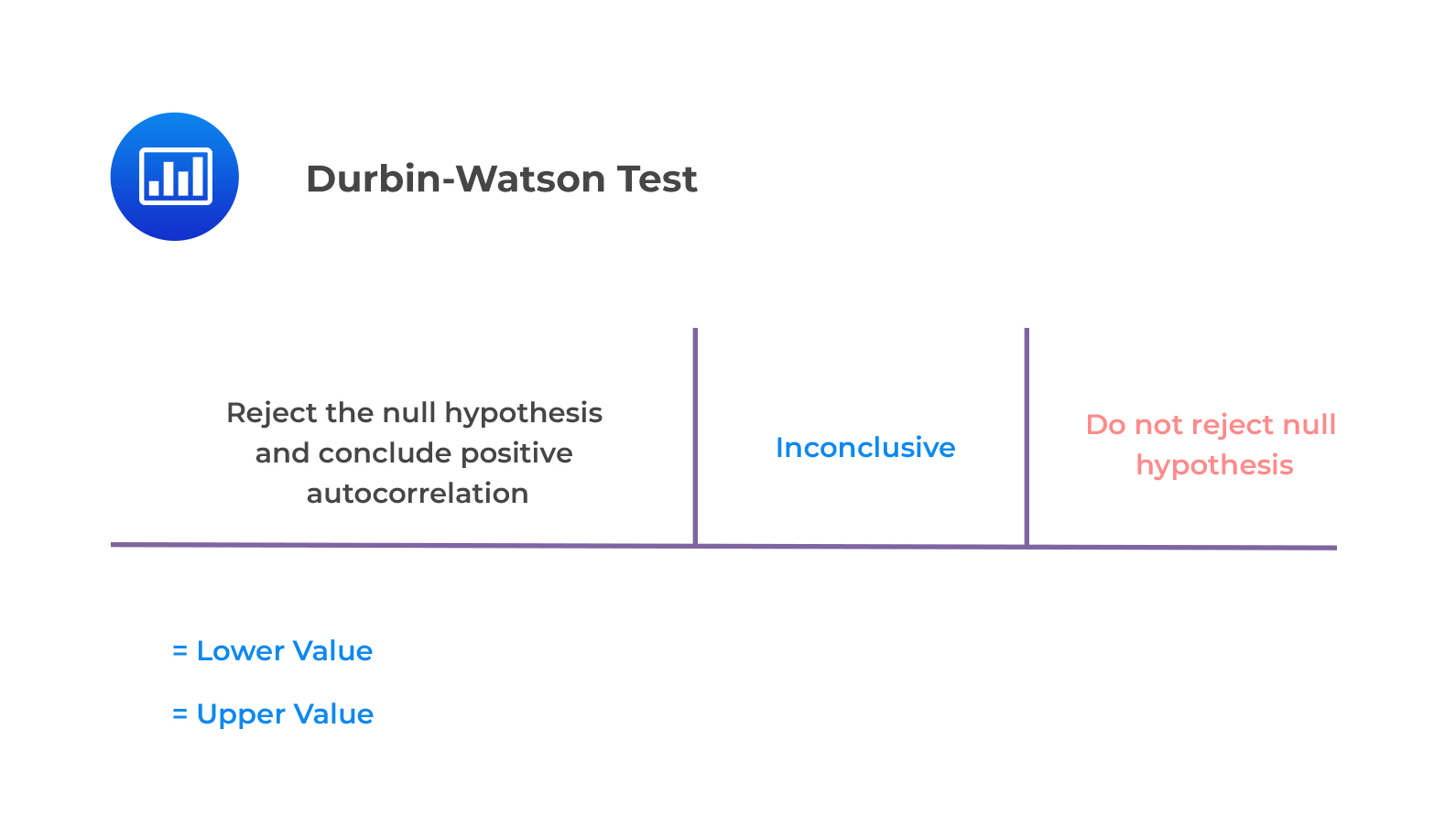
The null hypothesis of no positive autocorrelation is rejected if the Durbin–Watson statistic is below a critical value, \(d^{*}\), where \(d^{*}\) lies between an upper value \(d_{u}\) and a lower value \(d_{l}\) or outside of these values.

This is illustrated below.

Key Guidelines

• If \(d<d_{l}\), reject \(H_{0}: ρ =0\) (and so accept \(H_{1}:ρ >0\)).
• If \(d>d_{u}\), do not reject \(H_{0}:ρ =0\).
• If \(d_{l}< d<d_{u}\), the test is inconclusive.

Example: The Durbin Watson Test for Serial Correlation

Consider a regression output that includes two independent variables that generate a DW statistic of 0.654. Assume that the sample size is 15. Test for serial correlation of the error terms at the 5% significance level.

Solution

From the Durbin Watson table with \(n=15\) and \(k=2\), we see that \(d_{l}=0.95\) and \(d_{u}=1.54\). Since \(d=0.654<0.95=d_{l}\), we reject the null hypothesis and conclude that there is significant positive autocorrelation.

Correcting Autocorrelation

We can correct serial correlation by:

     i. Adjusting the coefficient standard errors for the regression estimates to take into account serial correlation. This is done using the Hansen method. This method can also be used to correct conditional heteroskedasticity. Hansen white standard errors are then used for hypothesis testing of the regression coefficient.

    ii. Modifying the regression equation to eliminate the serial correlation.

Question

Consider a regression model with 80 observations and two independent variables. Suppose that the correlation between the error term and a first lagged value of the error term is 0.15. The most appropriate decision is:

     A. Reject the null hypothesis of positive serial correlation.

     B. Fail to reject the null hypothesis of positive serial correlation.

     C. Declare that the test results are inconclusive.

Solution

The correct answer is B.

The test statistic is:

$$DW≈2(1-r)=2(1-0.18)=1.64$$

The critical values from the Durbin Watson table with \(n=80\) and \(k=2\) is \(d_{l}=1.59\) and \(d_{u}=1.69\)

Because \(1.64>1.59\), we fail to reject the null hypothesis of positive serial correlation.

Reading 2: Multiple Regression

LOS 2 (k) Explain the types of heteroskedasticity and how heteroskedasticity and serial correlation affect statistical inference.