Explain the Types of Heteroskedasticity and How It Affects Statistical Inference

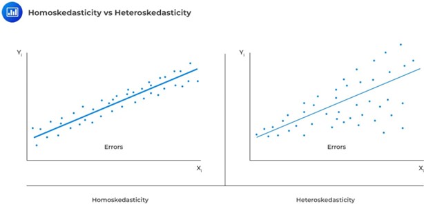
One of the assumptions underpinning multiple regression is that regression errors are homoscedastic. In other words, the variance of the error terms is equal for all observations:

$$ E\left(\epsilon_i^2\right)=\sigma_\epsilon^2,\ i=1,2,\ldots,n $$

In reality, the variance of errors differs across observations. This is known as heteroskedasticity.

Heteroskedasticity is a statistical concept that refers to the non-constant variance of a dependent variable. In other words, it occurs when the variability of a dependent variable is unequal across different values of an independent variable. This can often be seen in financial data, where the volatility of stock prices tends to be greater during periods of economic uncertainty. While heteroskedasticity can present challenges for statistical analysis, it can also provide valuable insights into the relationships between variables. For instance, by taking heteroskedasticity into account, economists can better understand how changes in one variable may impact the variability of another.

One way to test for heteroskedasticity is to look at the residuals from the regression. Uneven distribution of residuals (errors) could signify heteroskedasticity.

Types of Heteroskedasticity

There are two main types of heteroskedasticity: unconditional and conditional.

Unconditional heteroskedasticity occurs when the heterogeneity variance is not correlated with the values of the independent variables. Even though this goes against the homogeneity assumption, it does not produce major problems concerning statistical inference.

On the other hand, conditional heteroskedasticity happens when the error variance is dependent on the values of the independent variables. This creates considerable difficulties for statistical inference. Fortunately, there are many software programs that can identify and fix this issue.

Effects of Heteroskedasticity

Heteroskedasticity and the Consistency of Regression Parameter Estimators

One common misconception about heteroskedasticity is that it affects the consistency of regression parameter estimators. This is not the case. The ordinary least squares (OLS) estimators are still consistent, meaning that they will converge in probability to the true values of the parameters as the sample size increases. However, estimates of the variance and covariance of the estimators will be biased if heteroskedasticity is present in the data.

Heteroskedasticity and the F-test for Overall Significance

Another implication of heteroskedasticity is that it can make the F-test for overall significance unreliable. The F-statistic depends on the homoscedasticity assumption. So, if this assumption is violated, the test may not be valid.

Heteroskedasticity and t-tests for Individual Coefficients

Another common issue with heteroskedasticity is that it can introduce bias into estimators of the standard error of regression coefficients, making t-tests for individual coefficients unreliable. In particular, heteroskedastic errors tend to inflate t-statistics and underestimate standard errors.

Testing Heteroskedasticity

Breusch-Pagan Chi-square Test

The Chi-square test is used to test heteroskedasticity in a linear regression model. Trevor Breusch and Adrian Pagan developed the model in 1980. It is a generalization of the White test for heteroskedasticity, which was developed in 1950.

The test statistic is based on the regression of the squared residuals from the estimated regression equation on the independent variables. If the presence of conditional heteroskedasticity substantially explains the variation in the squared residuals, then the null hypothesis of no heteroskedasticity is rejected.

The test statistic is given by:

$$ \text{BP chi-square test statistic} = n \times R^2 $$

Where:

\(n\) = Number of observations.

\(R^2\) = Coefficient of determination from a regression of the squared residuals on the independent variables.

In case the null hypothesis of no heteroskedasticity is true, this statistic will be distributed as a chi-square random variable. We’ll have \(p\) degrees of freedom, where \(p\) is the number of independent variables in the model.

The Breusch-pagan test is a one-tailed test since we should mainly be concerned with heteroskedasticity for large test statistic values.

The Breusch-Pagan chi-square test can be used for heteroskedasticity in both pooled cross-sectional and time series data. In pooled cross-sectional data, each observation corresponds to a different individual, such as a different firm in a panel data set. In time series data, each observation corresponds to a different time period, such as a different year.

Example: Breusch-Pagan Chi-Square Test

Consider the multiple regression of the price of the USDX on inflation and real interest rates. The investor regresses the squared residuals from the original regression on the independent variables. The new \(R^2\) is 0.1874.

Test for the presence of heteroskedasticity at the 5% significance level.

Solution

The test statistic is:

$$ \begin{align*} \text{BP chi-square test statistic} & = n \times R^2 \\ & = 10 \times 0.1874 = 1.874 \end{align*} $$

The one-tailed critical value for a chi-square distribution with two degrees of freedom at the 5% significance level is 5.991.

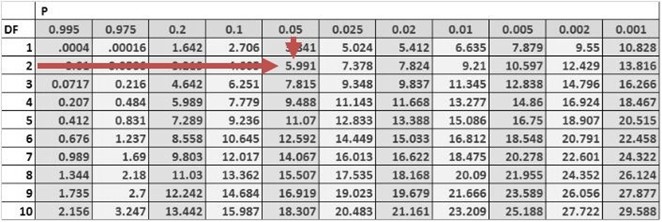
Therefore, we do not have sufficient evidence to reject the null hypothesis of no conditional heteroskedasticity. As a result, we conclude that the error term is not conditionally heteroskedastic.

Correcting Heteroskedasticity

In the investment world, it is crucial to correct heteroskedasticity. This is because it may change inferences about a particular hypothesis test, thus impacting an investment decision. One can apply two methods in the correction of heteroskedasticity: calculating robust standard errors and generalized least squares.

Computing Robust Standard Errors

The first method of correcting conditional heteroskedasticity is to compute robust standard errors. This means that the standard errors of the linear regression model’s estimated coefficients are adjusted to account for heteroskedasticity. This method is relatively easy to implement since many statistical software packages can automatically compute robust standard errors.

However, it does have some limitations. For example, robust standard errors can lead to conservative estimates of the coefficients—meaning coefficients may be underestimated.

Generalized Least Squares

The second method of correcting conditional heteroskedasticity is called generalized least squares. This method involves modifying the original equation to eliminate heteroskedasticity. The new, modified regression equation is then estimated under the assumption that heteroskedasticity is no longer a problem.

This method is more complex than computing robust standard errors, but it does not have the same limitations. For example, it does not necessarily lead to conservative estimates of the coefficients.