Theories of Growth

There are three growth theories based on the per capita growth in an economy:

1. The classical growth theory.
2. The neoclassical growth theory.
3. Endogenous growth theory.

The Classical Theory (Malthusian Theory)

Thomas Malthus developed the classical growth theory in 1798. The theory bases its argument on resource depletion and the growing population. Moreover, the production function in this theory is simple, with labor as a variable factor and land being a fixed factor.

The primary assumption in the Malthusian model is that population growth moves upwards when the level of per capita income increases beyond the subsistence income, i.e., the least amount of income to maintain life. Consequently, technological progress and labor expansion will raise labor productivity, which translates into higher population growth. However, diminishing marginal returns affect labor productivity. The extra output attributed to the rising workforce will finally drop to zero. In the long run, the population grows to the point where labor productivity drops, and per capita income returns to the subsistence point.

The classical model forecasts that technology adoption leads to a larger but not wealthier population in the long run. Therefore, the standard of living remains constant even with technological development and hence, no per capita output, making this theory a failure.

Reasons for Failure of Classical Growth Theory

1. The link between per capita income and population failed. Note that when the growth rate of per capita income increases, the population reduces instead of increasing.
2. Growth in per capita income has been viable due to technological progress being fast enough to counteract the diminishing marginal returns.

The Neoclassical Model

Robert Solow developed the neoclassic growth theory. The theory is based on Cobb-Douglas production. Note that the Cobb-Douglas Production function is presented as:

$$ Y=AF\left(K,L\right)=AK^\alpha L^{1-\alpha} $$

Where:

K= Capital stock.

L = Labor input.

A = Total factor productivity (TFP).

In the neoclassical growth theory, capital and labor are the varying factors affected by diminishing marginal productivity.

The Objective of Neoclassical Growth Rate

The neoclassical model evaluates the long-run growth rate of the per capita output concerning:

• Rate of technological progress.
• Population growth rate.
• Savings or investment rate.

While discussing the neoclassical model, two states of growth rate are considered:

1. Steady-state growth rate (equilibrium position).
2. When the economy has not achieved an equilibrium position.

Steady-state Rate of Growth

The neoclassical steady-state growth rate tries to find the equilibrium point at which the economy will shift. The equilibrium point is where the output-to-capital ratio is constant; the capital and output per worker grow simultaneously.

We analyze the neoclassical growth theory by considering the per capita Cobb-Douglas production functions:

$$ y=\frac{Y}{L}=Ak^\alpha $$

Where \(k=\frac{K}{L}\).

The rates of change of capital per worker are given by:

$$ \frac{\Delta k}{k}=\frac{\Delta K}{K}-\frac{\Delta L}{L} $$

And the rate of change of output per worker is given by:

$$ \frac{\Delta y}{y}=\frac{\Delta Y}{Y}-\frac{\Delta L}{L} $$

Deduced from the production function, the growth rate of output per worker can also be:

$$ \frac{\Delta y}{y}=\frac{\Delta A}{A}-\alpha\frac{\Delta k}{k}\ldots\ldots\ldots (\text{Eq 1}) $$

The physical capital of any economy will rise due to gross investment (I) and decline due to depreciation. Note that in a self-sufficient (closed) economy, domestic savings fund investment. Now, let’s be the proportion of income (Y) that is saved, then the gross investment (I) is given by:

$$ I=sY $$

Also, let \(\delta\) be the constant depreciation rate. Then, the change in physical capital stock is:

$$ \Delta K=sY-\delta K $$

Let the labor supply growth \(\frac{\Delta L}{L}=n\). Then,

$$ \begin{align*} \frac{\Delta k}{k} & =\frac{\Delta K}{K}-\frac{\Delta L}{L} \\ & =\frac{\Delta K}{K}-n \\ & =\frac{sY-\delta K}{K}-n \\ \Rightarrow\frac{\Delta k}{k} & =\frac{sY}{K}-\delta-n\ldots\ldots\ldots(\text{Eq 2}) \end{align*} $$

As stated previously, in an equilibrium position, the growth rate of capital per worker equals the growth rate of output per worker. Therefore:

$$ \frac{\Delta y}{y}=\frac{\Delta k}{k}=\frac{\Delta A}{A}-\alpha\frac{\Delta k}{k} $$

 Using Eq 2, we obtain:

$$ \frac{\Delta y}{y}=\frac{\Delta k}{k}=\frac{\frac{\Delta A}{A}}{1-\alpha} $$

Let TFP growth rate \(\frac{\Delta A}{A}\) be \(\theta\) that is, \(\theta=\frac{\Delta A}{A}\) then:

$$ \frac{\Delta y}{y}=\frac{\Delta k}{k}=\frac{\theta}{1-\alpha}\ldots\ldots\ldots(\text{Eq 3}) $$

From Eq 3, the steady-state (equilibrium position) of the sustainable growth rate of per capita output is a constant dependent on the TFP growth rate (\(\theta\)) and the output elasticity relative to capital (\(\alpha\)).

If we add the growth rate of labor \((\frac{\Delta L}{L}=n)\), we get the sustainable growth rate of output.

The growth rate of the production per capita (steady-state rate of growth of labor productivity) is:

$$ \frac{\mathrm{\Delta y}}{y}=\frac{\mathrm{\Delta k}}{k}=\frac{\theta}{1-\alpha} $$

The growth rate of output:

$$ \frac{{\Delta Y}}{Y}=\frac{\theta}{1-\alpha}+n $$

At this point, we have reached a significant result of the neoclassical model. Note that \(\frac{\theta}{1-\alpha}\) is also a steady-state growth rate of labor productivity. The last formulas are in sync with the labor productivity accounting equation:

$$ \begin{align*} & \text{Growth rate in potential GDP} \\ & = \text{Growth rate of the labor force over a long-term period} \\ & + \text{Growth rate of labor productivity over a long-term period.} \end{align*} $$

Now, consider Eq 2. If we substitute \(\frac{\Delta k}{k}=\frac{\theta}{1-\alpha}\) on its left-hand side, the rearrangement gives the equilibrium output-to-capital ratio \((\Psi)\). That is,

$$ \begin{align*} \frac{\Delta k}{k} & =\frac{sY}{K}-\delta-n \\ =\frac{\theta}{1-\alpha} &=\frac{sY}{K}-\delta-n \\ \Rightarrow\frac{sY}{K} &=\left(\frac{\theta}{1-\alpha}\right)+\delta+n \\ \therefore\Psi =\frac{Y}{K} &=\frac{1}{s}\left[\left(\frac{\theta}{1-\alpha}\right)+\delta+n\right]\ldots\ldots\ldots(\text{Eq 4}) \end{align*} $$

In an equilibrium position, the output-to-capital ratio is constant, and the capital to labor (\(k\)) ratio and labor productivity (\(y\)) grow at the same pace, evidenced by \(\left(\frac{\theta}{1-\alpha}\right)\). Moreover, the marginal product of capital \([\alpha\left(\frac{Y}{K}\right)]\) is constant and equal to the real interest rate in the market.

Example: Calculating Steady Rate of Growth in Neoclassical Model

A developed country has a labor cost in total factor cost of 45%, a TFP growth rate of 3%, and a labor growth rate of 2%. Using the neoclassical model, the steady rate of growth for this country  is closest to:

Solution

From the neoclassical model, the steady growth rate is given by:

$$ \frac{\Delta Y}{Y}=\frac{\theta}{1-\alpha}+n $$

From the information given,

\(\theta\) = Growth rate in TFP = 3% = 0.03

\(1-\alpha\) = Labor share of output = 45% = 0.45

n = Growth rate of the labor force = 2% = 0.02

So,

$$ \frac{\Delta Y}{Y}=\frac{0.03}{0.45}+0.02=0.08667=8.667\% $$

An alternative method of grasping the equilibrium position is rewriting Eq 4 to savings or investment equation as:

$$ sy=\left[\left(\frac{\theta}{1-\alpha}\right)+\delta+n\right]k $$

From the equation above, the steady-state rate of growth is reached where the actual gross investment per worker created in the economy and savings are just enough to:

1. Give capital to new workers incorporated into the workforce at a rate of \(n\).
2. Replace depreciation (for example, wearing and tearing of equipment).
3. Increase physical capital stock at a rate of \(\left[\frac{\theta}{1-\alpha}\right]\) to keep the marginal product of capital equal to the rental price (r) of money.

The steady-state rate of growth in the neoclassical model is shown below.

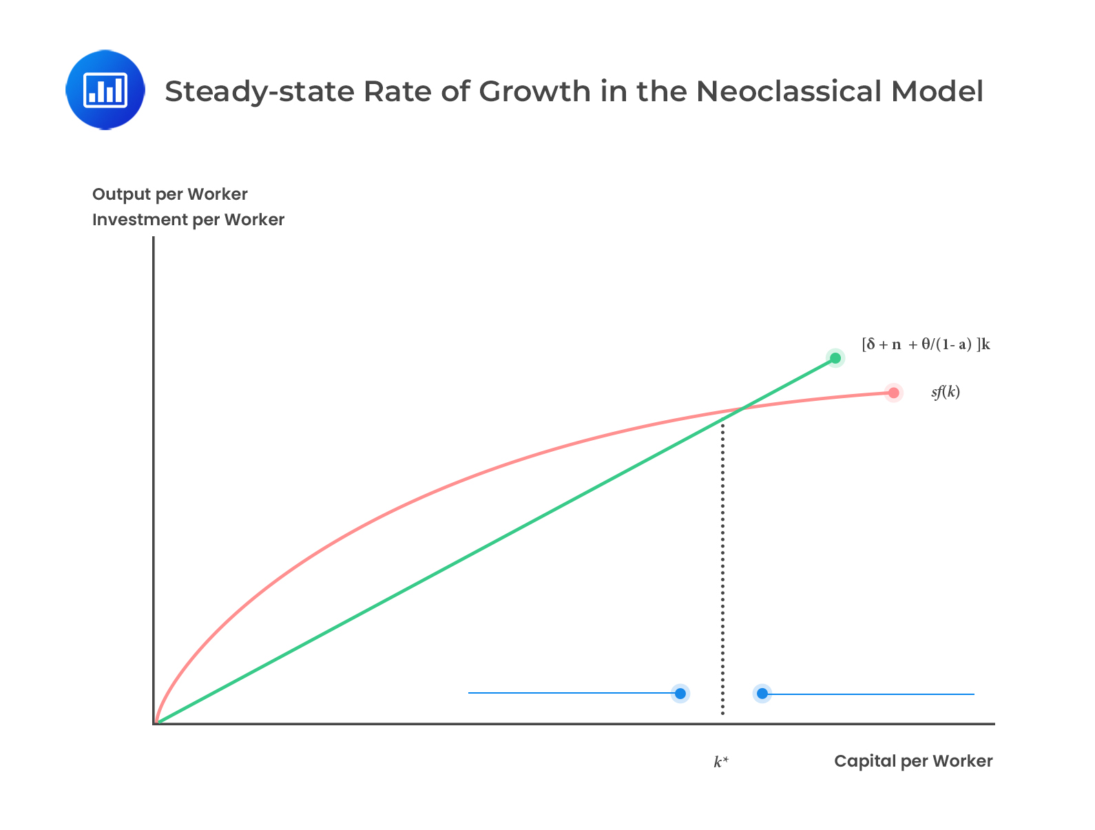The straight line represents the amount of investment necessary for the required physical capital growth rate\(\left[\left[\left(\frac{\theta}{1-\alpha}\right)+\delta+n\right]k\right]\) with the gradient equal to \(\left[\left(\frac{\theta}{1-\alpha}\right)+\delta+n\right]\). The curved line (due to diminishing marginal returns) represents the actual investment \((sf(k))\) by each worker. It is determined by the rate of saving and the production function.

The point where the required and the actual investment lines intersect is called the steady state or the equilibrium position.

Impact of Neoclassical Model Parameters on the Steady State Rate of Growth

Saving Rate (s)

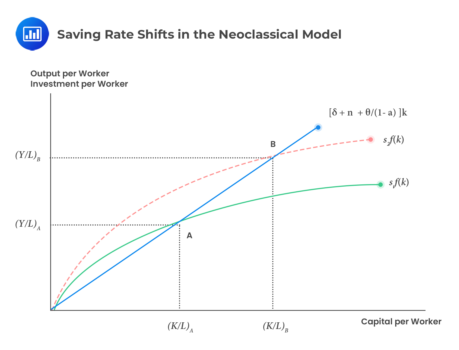
A high saving rate leads to a higher capital-to-labor ratio (\(k\)) and labor productivity (\(y\)) due to more savings or investments at each level of output.

Graphically, a high saving rate shifts the \(sf(k)\) curve upwards, hence the equilibrium points.

Depreciation Rate, (\(\delta\))

When the depreciation rate drops, the equilibrium capital-to-labor ratio and output per worker decrease since a given gross saving rate creates less capital accumulation. Graphically, it increases the slope of the required investment and hence changes the equilibrium position.

Labor Force Growth, (n)

When the growth rate of the labor force increases, the equilibrium capital-to-labor ratio decreases since the corresponding rise in the steady-state growth rate of capital is necessary. Graphically, when the slope of the required investment increases, it also shifts the equilibrium positions.

Growth in TFP, (\(\theta\))

When there is a rise in the growth rate of TFP, the steady-state capital-to-labor ratio and output per worker is reduced for a provided size of labor and TFP. Graphically, the effect is the same as that of labor force growth.

Neoclassical Model When the Economy Has Not Achieved Equilibrium Position

An economy experiences a higher or slower growth relative to a steady state when transitioning to stable growth alignment.

Using Eq 1, Eq 2, and Eq 3, we can present the growth rate of output per capita as:

$$ \frac{\Delta y}{y}=\frac{\theta}{1-\alpha}+\alpha s\left(\frac{Y}{K}-\Psi\right)=\frac{\theta}{1-\alpha}+\alpha s\left(\frac{y}{k}-\Psi\right)\ldots\ldots\ldots (\text{Eq 5}) $$

And growth to labor ratio as:

$$ \frac{\Delta k}{k}=\frac{\theta}{1-\alpha}+s\left(\frac{Y}{K}-\Psi\right)=\frac{\theta}{1-\alpha}+s\left(\frac{y}{k}-\Psi\right)\ldots\ldots\ldots (\text{Eq 6}) $$

The second equality of (Eq 5) and (Eq 6) is true because of the definition of \(y\) and \(k\), and it implies that \(\frac{Y}{K}=\frac{y}{k}\)

Graphically, the relationships in the neoclassical growth theory are shown below.

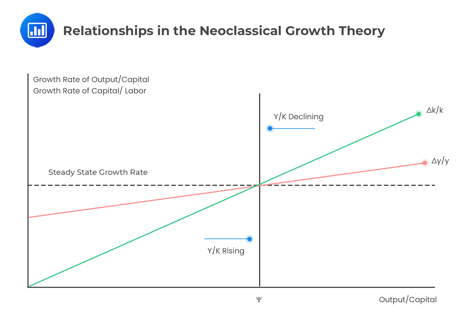When the output-to-capital ratio is higher than the equilibrium level (\(\Psi\)), Eq 5 and Eq 6 are positive. Moreover, the growth rates of the production per capita and the capital-to-labor ratios are higher than the steady-state \(\left[\frac{\theta}{1-\alpha}\right]\). This represents a situation where the actual savings or investments are higher than the required investment. The trend rate of capital deepening causes the trend in per capita output.

Conversely, if the output-to-capital ratio is below the state, the actual investment is insufficient to maintain the capital-to-labor ratio trend. Besides, the output per capita and capital-to-labor ratios grow more slowly.

Implications of the Neoclassical Model

1. Capital Accumulation

In the long run, capital accumulation will affect economic growth but not the level of output. A growing economy will always move towards the attainment of a steady state of growth. It is imperative to remember that the output growth rate is not dependent on accumulated capital.

2. Capital Deepening vs. Technology

For long-term sustainable economic growth to occur, an economy cannot rely on capital-deepening investments alone. Diminishing marginal returns will occur when the increase of some inputs is not the same as other inputs. Without improvements in TFP per capita, the output and labor productivity growth will reduce. Due to diminishing marginal returns to capital, only growth in technology will lead to the sustainable growth of potential GDP per capita.

3. Convergence

The high marginal productivity of capital and high saving rates in developing countries should make the growth rates of such countries higher than that of their developed counterparts. Therefore, a convergence of per capita incomes should exist between developed and developing countries over time.

4. Effects of savings on growth

In the short run, higher savings will lead to an increment in the economy’s growth rate. In fact, the growth will exceed the steady-state growth rate, but once the transition period is over, it will return to a balanced state. Higher levels of productivity are experienced during the transition period. Once steady-state growth is reached, the economy no longer depends on the high savings rate.

Endogenous Growth Theory

The endogenous growth theory explains technological progress rather than taking it as an external (exogenous) factor. According to the model, self-sufficient economic growth results from the model’s outcome, and the economy does not converge to an equilibrium position of the growth rate. Contrary to what is the case in the neoclassical model, there is no diminishing marginal capital for the whole economy. Therefore, a permanent increase in the saving rate increases economic growth.

The production function in the endogenous growth theory’s production function is a straight line (unlike that of the neoclassical model, which is curved) given by:

$$ y_e=f\left(k_e\right)=ck_e \ldots\ldots\ldots  (\text{Eq 7}) $$

Where:

\(e\) represents the endogenous growth model.

\( k_e \) = Capital per worker.

\( y_e \) = Output per worker (proportional to capital per worker).

\(c\) = Constant marginal product of capital in the whole economy.

The endogenous growth model postulates that the output-to-capital ratio (\(c\)) and the output per worker (\(y_e\)) grow at the same pace as the capital per worker (\(k_e\)). It, therefore, follows that faster (slower) accumulation of capital results in faster (slower) growth in output per capita.

Now, if (Eq 7) is in (Eq 2), we get:

$$ \frac{\Delta y_e}{y_e}=sc-\delta-n $$

Note that the right-hand side of the above equation is a constant, implying that it applies to both the long-run and the short-run growth rates. Moreover, an increased saving rate (\(s\)) results in a permanently high growth rate. The equation above is the result of the endogenous growth theory.

Question

An economy has a per capita income constant growth rate of 4%, a saving rate of 20%, an output-to-capital ratio of 0.65, depreciation of 10%, and a labor force growth rate of 1.5%. The saving rate increases by 4.5%. According to endogenous growth theory, the new steady growth rate is closest to:

1. 4.325%.
2. 4.252%.
3. 4.425%.

Solution

The correct answer is C.

From the information given in the question,

$$ s = 0.02 + 0.045=0.245 $$

\(\delta\) = 0.1.

\(n\) =0.015.

Output-to-capital ratio (which is constant for endogenous growth theory), \(c\) = 0.65.

Under the endogenous growth theory, the new growth rate of the per capita income is given by:

$$ \frac{\Delta y_e}{y_e}=sc-\delta-n=0.245\times0.65-0.10-0.015=0.04425=4.425\% $$

Reading 9: Economic Growth

LOS 9 (i) Compare classical growth theory, neoclassical growth theory, and endogenous growth theory.