


Interest Rate Forward and Futures Cont ...
The most used interest rate in the derivatives market is the LIBOR which... Read More

Serial correlation, also known as autocorrelation, occurs when the regression residuals are correlated with each other. In other words, it occurs when the errors in the regression are not independent of each other. This can happen for various reasons, including incorrect model specification, not randomly distributed data, and misspecification of the error term.
This is common with time-series data. One example of serial correlation is found in stock prices. Stock prices tend to go up and down together over time, which is said to be “serially correlated.” This means that if stock prices go up today, they will also go up tomorrow. Similarly, if stock prices go down today, they are likely to go down tomorrow. The degree of serial correlation can be measured using the autocorrelation coefficient. The autocorrelation coefficient measures how closely related a series of data points are to each other.
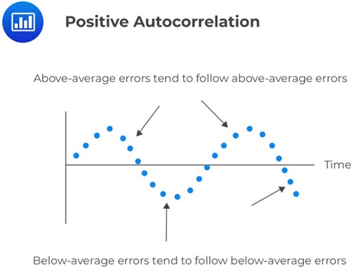
Positive serial correlation occurs when a positive error for one observation increases the chance of a positive error for another observation. In other words, if there is a positive error in one period, there is a greater likelihood of a positive error in the next period as well. Positive serial correlation also means that a negative error for one observation increases the chance of a negative error for another observation. So, if there is a negative error in one period, there is a greater likelihood of a negative error in the next period.
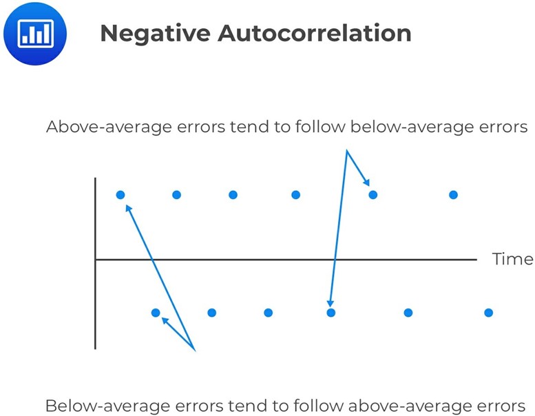
A negative serial correlation occurs when a positive error for one observation increases the chance of a negative error for another observation. In other words, if there is a positive error in one period, there is a greater likelihood of a negative error in the next period. A negative serial correlation also means that a negative error for one observation increases the chance of a positive error for another observation. So, if there is a negative error in one period, there is a greater likelihood of a positive error in the next period.
The first thing to understand about serial correlation is that it does not cause bias in the regression coefficient estimates. However, the positive serial correlation will inflate the F-statistic to test the overall significance of the regression because the mean squared error (MSE) will tend to underestimate the population error variance. This increases Type I errors (rejecting the null hypothesis when it is true). In other words, you are more likely to reject the null hypothesis when it is true if there is a positive serial correlation in your data.
On the other hand, a negative serial correlation will deflate the F-statistic because the MSE will tend to overestimate the population error variance. This decreases Type I errors but increases Type II errors (the failure to reject the null hypothesis when it is false). So, you are more likely to fail to reject the null hypothesis when it is false if there is a negative serial correlation in your data.
The positive serial correlation makes the ordinary least squares standard errors for the regression coefficients underestimate the true standard errors. Moreover, it leads to small standard errors of the regression coefficient, making the estimated t-statistics seem statistically significant relative to their actual significance.
In addition to affecting significance tests, serial correlation affects confidence intervals and hypothesis tests for individual coefficients. The positive serial correlation makes the OLS standard errors for the regression coefficients underestimate the true standard errors. Moreover, it leads to small standard errors of the regression coefficient, making the estimated t-statistics seem statistically significant relative to their actual significance.
The first step of testing for serial correlation is plotting the residuals against time. The other most common formal test is the Durbin-Watson test.
The Durbin-Watson test is a statistical test used to determine whether or not there is a serial correlation in a data set. It tests the null hypothesis of no serial correlation against the alternative positive or negative serial correlation hypothesis. The test is named after James Durbin and Geoffrey Watson, who developed it in 1950.
The Durbin-Watson Statistic (DW) is approximated by:
$$ DW = 2(1 − r) $$
Where:
\(r\) is the sample correlation between regression residuals from one period and the previous period.
The test statistic can take on values ranging from 0 to 4. A value of 2 indicates no serial correlation, a value between 0 and 2 indicates a positive serial correlation, and a value between 2 and 4 indicates a negative serial correlation:
If there is no autocorrelation, the regression errors will be uncorrelated, and thus \(DW = 2\)
$$ DW = 2(1 − r) = 2(1 − 0) = 2 $$
For positive serial autocorrelation, \(DW < 2\). For example, if serial correlation of the regression residuals = 1, \(DW = 2(1 − 1) = 0\).
To reject the null hypothesis of no serial correlation, we need to find a critical value lower than our calculated value of d*. Unfortunately, we cannot know the true critical value, but we can narrow down the range of possible values.
Define \(d_l\) as the lower value and \(d_u\) as the upper value:
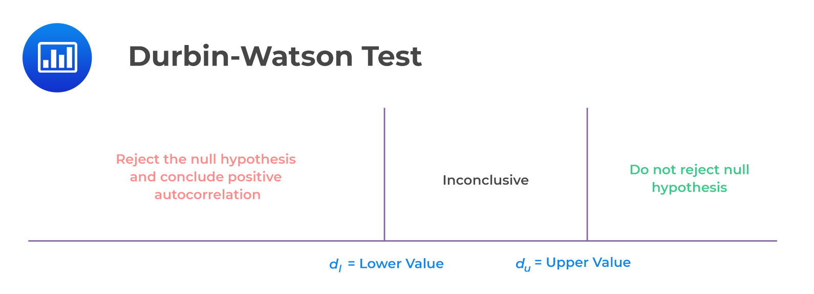
Consider a regression output with two independent variables that generate a DW statistic of 0.654. Assume that the sample size is 15. Test for serial correlation of the error terms at the 5% significance level.
From the Durbin-Watson table with \(n = 15\) and \(k = 2\), we see that \(d_l = 0.95\) and \(d_u = 1.54\). Since \(d = 0.654 < 0.95 = d_l\), we reject the null hypothesis and conclude that there is significant positive autocorrelation.
One way is to adjust the coefficient standard errors for the regression estimates to account for serial correlation. This is done using the Hansen method or the Newey-West estimator.
Danish statistician Thorvald Hansen developed the Hansen method in the early 20th century. Researchers have since refined the technique. The Hansen method proposes the estimation of the degree of autocorrelation in the data under review as the first step in autocorrelation correction. The standard errors are then adjusted accordingly. This correction can be important in fields such as econometrics, where even small inaccuracies can lead to large errors in estimates. While the Hansen method is not perfect, it remains one of the most reliable tools for dealing with autocorrelation.
Economists Whitney Newey and Ken West developed the Newey-West estimator. This method is widely used in econometrics and finance. It works by creating a weighting matrix that assigns lower weights to observations more likely to correlate with each other. This technique can be used with both cross-sectional data and time-series data.
Another way to correct serial correlation is to modify the regression equation. This can be done by adding a lag term, which represents the value of the dependent variable at a previous period. By including this lag term, we can account for any correlations that may exist between the dependent variable and the error terms. As a result, our estimates will be more accurate, and we will be less likely to make a Type I error.
Besides, there are several other methods that can be used to correct for serial correlation, including the use of instrumental variables and panel data methods.
Question
Consider a regression model with 80 observations and two independent variables. Assume that the correlation between the error term and the first lagged value of the error term is 0.18. The most appropriate decision is:
- reject the null hypothesis of positive serial correlation.
- fail to reject the null hypothesis of positive serial correlation.
- declare that the test results are inconclusive.
Solution
The correct answer is C.
The test statistic is:
$$ DW \approx 2(1 − r) = 2(1 − 0.18) = 1.64 $$
The critical values from the Durbin Watson table with \(n = 80\) and \(k = 2\) is \(d_l = 1.59\) and \(d_u = 1.69\).
Because 1.69 > 1.64 > 1.59, we determine the test results are inconclusive.
Regression analysis can be one of the more technical areas of the CFA Level II curriculum. Practicing topics like the Durbin-Watson test and correcting autocorrelation can help you apply formulas accurately under exam pressure.
Prepare smarter with CFA Level II question bank practice designed to reinforce key Quantitative Methods concepts.
Practice CFA Level II time-series questions covering serial correlation, regression errors, hypothesis testing, and step-by-step exam-style solutions.
Offered by AnalystPrep


Get Ahead on Your Study Prep This Cyber Monday! Save 35% on all CFA® and FRM® Unlimited Packages. Use code CYBERMONDAY at checkout. Offer ends Dec 1st.