


Construction of Commodity Indexes
Commodity indexes have been created to portray the aggregate movement of commodity prices,... Read More

In statistics, regression analysis is a method of modeling the relationships between a dependent variable (also called an outcome variable) and one or more independent variables (also called predictor variables). Regression analysis aims to find the best-fitting line or curve that describes how the dependent variable changes as the independent variable changes.
A crucial part of regression analysis entails identifying the data points which are most influential in determining the shape of the best-fitting line or curve. These data points are known as influential data points. An influential data point has a significant effect on the fitted or predicted values of the model. Influential data points can greatly impact the regression analysis results, even if they are not necessarily representative of the entire dataset.
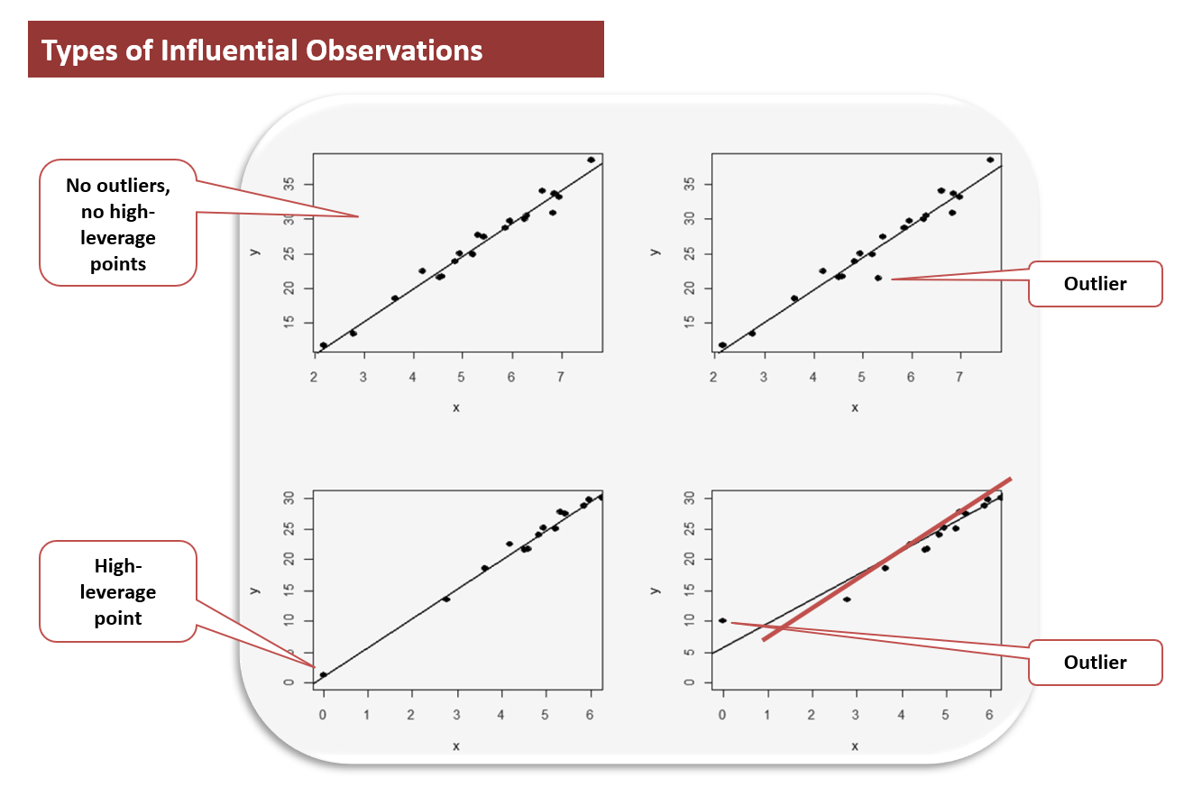
There are a few different types of data points that can be influential in a multiple regression analysis. These include high-leverage points and outliers.
A high-leverage point is a data point with an extreme value of the independent (explanatory) variable. High-leverage points have a relatively large influence on the fitted values of the regression line. This means that if you were to remove a high-leverage point from your dataset, the regression line would change quite a bit.
An outlier is a point with a larger or smaller y value than the model suggests. Outliers don’t fit well with the rest of the dataset. They can either be positive or negative outliers. Positive outliers are values that are too high, while negative outliers are values that are too low.
There are a number of different methods for detecting influential data points in multiple regression. The two most common methods are leverage and Cook’s distance.
Leverage, \(h_{ii}\), is a measure of how far away an individual data point is from the mean of the rest of the data. For a particular independent variable, leverage measures the distance between the ith observation of that variable and the mean of the variable across \(n\) observations. Leverage lies between 0 and 1. The sum of individual leverages for all observations is \(k + 1\), where \(k\) is the number of independent variables.
So, what’s the threshold for an observation to be considered an “influential” data point? As a general rule of thumb, an observation is potentially influential if its leverage exceeds \(3[\frac {(k+1)}{n}]\), where \(k\) is the number of independent variables and \(n\) is the number of observations in the data set. For example, if you have a dataset with 50 observations and 10 independent variables, any observation with a leverage greater than 0.66 could be considered potentially influential.
A data point with high leverage can significantly impact the overall trend, even if its value is not particularly extreme.
A studentized residual, \(t_i^\ast\), is a statistic that is used to identify outliers in a dataset. It is a residual that has been scaled by an estimate of its standard deviation. It is calculated by dividing the residual (the difference between the actual value and the predicted value) by the standard deviation of the residuals.
$$ t_i^\ast=\frac{e_{i^\ast}}{s(e^\ast)}=e_i\sqrt{\frac{n-k-1}{SSE\left(1-h_{ii}\right)-e_i^2}} $$
Where:
\(e_{i^\ast} =\) Residual with the \(i^\text{th}\) observation deleted.
\(s_e^\ast =\) Standard deviation of residuals.
\(k =\) Number of independent variables.
\(n =\) Total number of observations.
\(SSE =\) Sum of square errors of the original regression model.
\(h_{ii} =\) Leverage value for the ith observation.
When interpreting the studentized residual, it is important to remember that a zero value indicates that the data point is not an outlier. Positive values indicate that the data point is above the regression line, while negative values indicate that the data point is below the regression line. Generally speaking, a studentized residual should be considered significant if it is greater than 2 in absolute value.
A more reliable way to determine whether an observation is influential using the studentized residual is to compare it with the critical value of the t-distributed statistic with \(n – k – 2\) degrees of freedom at the selected significance level. The observation is considered influential if the studentized residual is greater than the critical value.
Cook’s distance measures the influence of each observation on the estimated regression coefficients. Statistician R. Dennis Cook developed Cook’s distance in 1970. Cook’s distance measures how much the estimate of the regression coefficients would change if a given observation were removed from a data set. In other words, it quantifies how “important” each observation is in relation to the fit of a model. The larger the value of Cook’s distance, the greater the influence of the observation. Cook’s distance formula is as follows:
$$ D_i=\frac{(y_i-{\hat y}_i)^2}{k\times MSE}\left(\frac{h_{ii}}{(1-h_{ii})^2}\right)=\frac{e_i^2}{k\times M S E}\left(\frac{h_{ii}}{(1-h_{ii})^2}\right) $$
Where:
\(e_i =\) Residual for observation \(i\).
\(K\ =\) Number of independent variables.
\(MSE =\) Mean square error of the estimated regression model.
\(h_{ii} =\) Leverage value for observation \(i\).
Data points with a Cook’s distance greater than \(1\) or \(2\sqrt{\frac {k}{n}}\) are considered to be influential. This means they can potentially skew the results of the analysis. Data points with a Cook distance between 0.5 and 1 are considered moderately influential. This means they may not significantly impact the results but could still be worth considering. Data points with a Cook distance of less than 0.5 are not considered influential, so they can safely be ignored when analyzing the data.
Reading 4: Extensions of Multiple Regression
Los 4 (a) Describe Influence analysis and methods of detecting influential data points
Strengthen your CFA Level II quantitative methods skills with exam-style questions on regression diagnostics, leverage, and influential observations.
Offered by AnalystPrep


Get Ahead on Your Study Prep This Cyber Monday! Save 35% on all CFA® and FRM® Unlimited Packages. Use code CYBERMONDAY at checkout. Offer ends Dec 1st.