


Standard 1(A) – Knowledge of the Law
Members and Candidates must understand and comply with all applicable laws, rules, and... Read More

Historical simulation employs randomness by drawing returns from historical data randomly, instead of following each period chronologically. An election can be made on whether to sample from the historical returns with or without replacement. Analysts prefer drawing samples from historical returns without replacement since the number of simulations is larger, in this case, than the historical data size. Note that random sampling with replacement is also known as bootstrapping.
Let us use the factor allocation strategies for eight-factor portfolios to illustrate and interpret a simulation.
$$\small{\begin{array}{l|c|c|c|c|c|c|c}\textbf{Simulation} & \textbf{Month} & {\textbf{Random}\\ \textbf{no}} & {\textbf{Month}\\ \textbf{no}} & {\textbf{Earnings}\\ \textbf{Yield}} & {\textbf{Book-to-}\\ \textbf{Market}} & {\textbf{Earnings}\\ \text{Growth}} & \textbf{Momentum} \\ \hline1 & 31/10/2006 & 0.595441 & 223 & 2.5\% & 0.3\% & -0.8\% & 0\% \\ \hline 2 & 31/5/1998 & 0.32574 & 122 & 0.1\% & 0.8\% & -0.2\% & -0.5\% \\ \hline 3 & 31/3/2012 & 0.76896 & 288 & -2\% & 0.6\% & 1.7\% & 1.8\% \\ \hline4 & 31/3/2016 & 0.89712 & 336 & 2.6\% & 2.5\% & -0.4\% & -1.5\% \\ 5 & 30/6/2002 & 0.45657 & 171 & 6.5\% & -3.4\% & 1.8\% & 2.4\%\\ \end{array}}$$
$$\small{\begin{array}{l|c|c|c|c|c|c|c} \textbf{Simulation} & \textbf{Month} & {\textbf{Random}\\ \textbf{no}} & {\textbf{Month}\\ \textbf{no}} & {\textbf{Earnings}\\ \textbf{Revision}} & \textbf{ROE} & \textbf{Debt/Equity} & {\textbf{Earnings}\\ \textbf{Quality}} \\ \hline 1 & 31/10/2006 & 0.595441 & 223 & -0.75\% & 2.5\% & 0.5\% & -0.6\% \\ \hline 2 & 31/5/1998 & 0.32574 & 122 & -0.1\% & -0.1\% & 0.3\% & 1.6\% \\ \hline 3 & 31/3/2012 & 0.76896 & 288 & 2\% & -0.6\% & -2.02\% & -0.9\% \\ \hline 4 & 31/3/2016 & 0.89712 & 336 & -1.6\% & 1.5\% & -1.2\% & 1.4\% \\ \hline 5 & 30/6/2002 & 0.45657 & 171 & 2.5\% & 6.4\% & -0.8\% & 1.3\%\\ \end{array}}$$
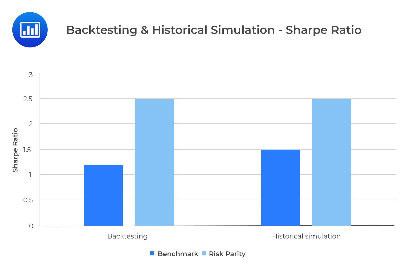
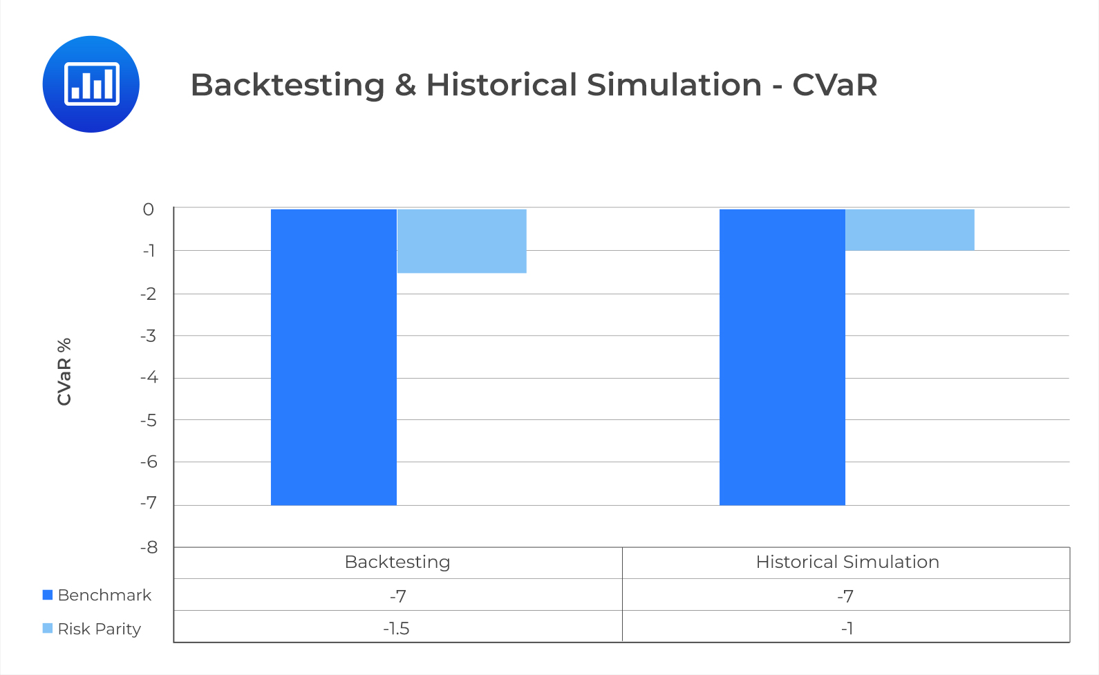
From Exhibit 5, the Sharpe ratios of the RP and BM strategies are in line with those of the rolling window backtesting. In both approaches, the BM portfolio is outperformed by the RP portfolio according to the Sharpe ratio. For both approaches, RP carries less substantial downside risk than the BM portfolio.
One problem with historical simulation is that it uses past data that may not represent the future. To address this problem, we will use the Monte Carlo simulation. The steps for both methodologies are similar, with a few key differences which we will highlight in this section. First, we have to specify a functional form for each key decision variable. Exploratory data analysis is often important here. The usefulness of Monte Carlo simulation depends on how well the functional forms reflect the true distribution of the underlying data.
A few key considerations need to be made before we can finalize our choice of functional forms.
Using the RP and BM strategies, the Monte Carlo simulation can be carried out as follows:
$$\small{\begin{array}{l|c|c|c|c|c|c|c|c}{\textbf{Simulation}\\ \textbf{no}} & {\textbf{Earnings}\\ \textbf{Yield}} & {\textbf{Book-to-}\\ \textbf{Market}} & {\textbf{Earnings}\\ \textbf{Growth}} & \textbf{Momentum} & {\textbf{Earnings}\\ \textbf{Revision}} & \textbf{ROE} & \textbf{Debt/Equity} & {\textbf{Earnings}\\ \textbf{Quality}} \\ \hline 1 & -3\% & -3.2\% & -0.3\% & 0.7\% & 2.4\% & -3.3\% & -1.8\% & 2\% \\ \hline 2 & 0\% & 3.7\% & 1\% & -0.5\% & 1\% & -2.3\% & -3.5\% & -0.2\% \\ \hline 3 & 0.8\% & -2\% & 3\% & 3.9\% & 2.6\% & 1.3\% & -0.9\% & 0\% \\ \hline 4 & 9.5\% & -0.4\% & 1.2\% & 3.8\% & -1\% & 7.7\% & -3.8\% & 1.7\% \\ \hline 5 & 1.8\% & 0.3\% & 2.9\% & -0.3\% & 3.2\% & 0.3\% & -1\% & 0.3\%\\ \end{array}}$$
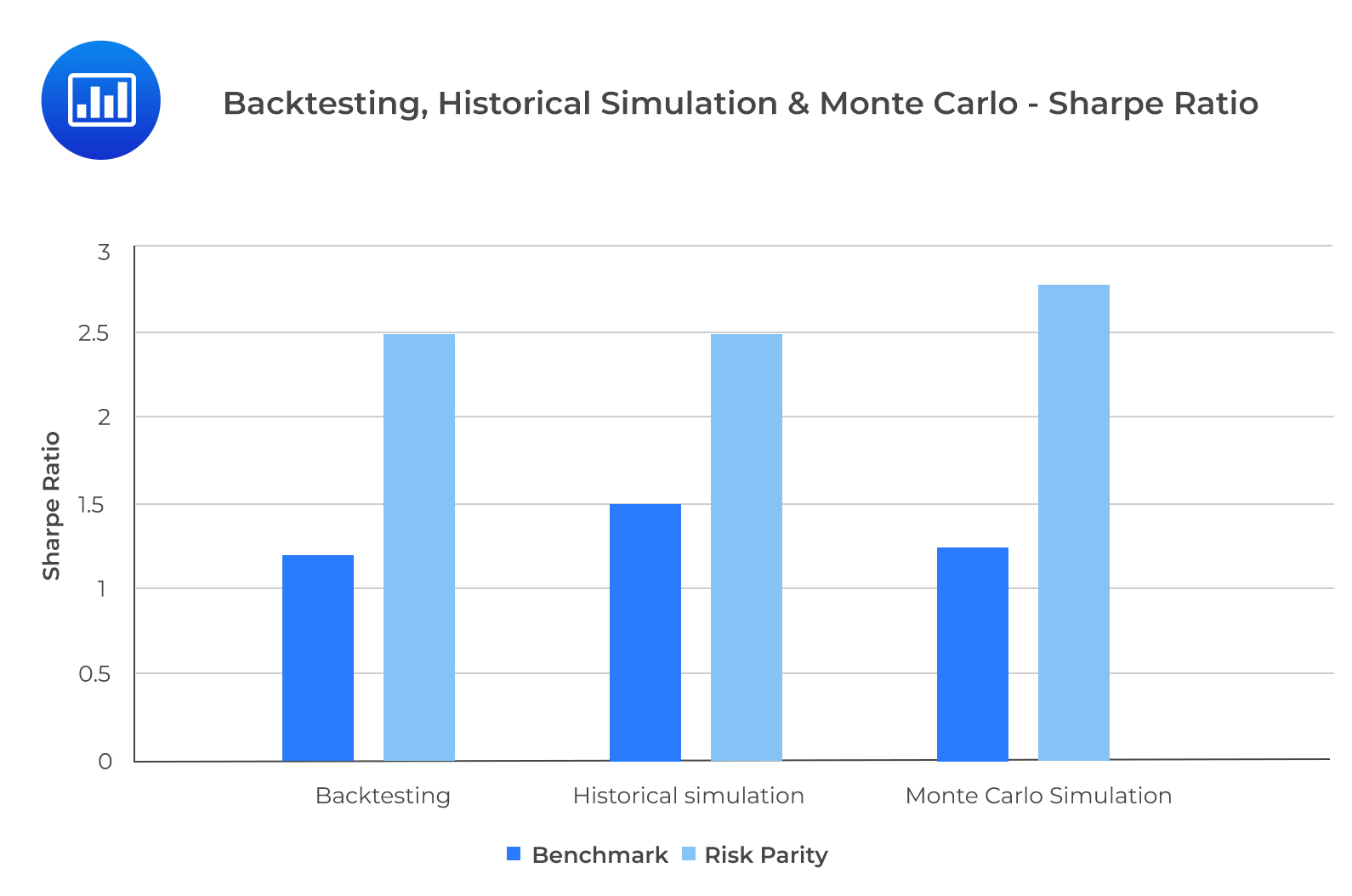
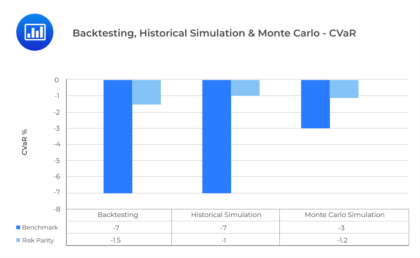
From exhibit 7, we can see that the RP strategy outperformed the BM strategy according to the Sharpe ratio in all three approaches. The CVar is slightly more sensitive to randomness. Compared to rolling window backtesting and historical simulation, it is under the Monte Carlo simulation that the downside risk is most understated for the BM strategy. This is because the factor returns for the Monte Carlo simulation are negatively skewed with excess kurtosis. The underestimation of risk only appears for the BM strategy because the correlations and the factor risks are not properly accounted for in the equal weighing scheme.
Question
What could be the most likely reason why the downside risk of the benchmark strategy would be underestimated under the Monte Carlo simulation:
- BM strategy is robust to non-normal factor distribution.
- The correlations and the factor risks are properly accounted for in the equal weighing scheme.
- The correlations and the factor risks are not properly accounted for in the equal weighing scheme.
Solution
The correct answer is C.
The underestimation of risk only manifests in the BM strategy because the correlations and the factor risks are not properly accounted for in the equal weighing scheme.
A is incorrect. The risk parity strategy is robust to a non-normal factor return distribution.
B is incorrect. The underestimation of downside risk would not occur if the correlations and the factor risks were accurately accounted for.
Reading 42: Backtesting and Simulation
LOS 42 (g) Explain inputs and decisions in simulation and interpret a simulation.
Review inputs and decisions in simulation with CFA Level 2 study notes, practice questions, mock exams, and video lessons designed to strengthen your exam preparation.
Offered by AnalystPrep


Get Ahead on Your Study Prep This Cyber Monday! Save 35% on all CFA® and FRM® Unlimited Packages. Use code CYBERMONDAY at checkout. Offer ends Dec 1st.