Sensitivity Analysis

Monte Carlo simulation fits the factor returns to a multivariate normal distribution but fails to account for negative skewness and fat tails. This is what informs the need for a sensitivity analysis. The analysis is done by fitting a different distribution to the factor return data and repeating the Monte Carlo simulation. Sensitivity analysis explores how a target variable is affected when the input variables are changed. Sensitivity analysis can, as such, help managers comprehend the potential risks and returns of their investment strategies.

Multivariate Student’s t-distribution is an alternative that can be used because of its ability to account for the skewness and the excess kurtosis observed in asset and factor return data. This alternative calls for estimating a larger number of parameters. Further, it is more mathematically complex. To determine the sensitivity of our target variable to the new factor return distribution, we follow the same steps we did follow in the previous section with two slight differences. In step 4, we calibrate our model to a multivariate skewed t-distribution. In addition, in step 5, 800 sets of factor returns from this new distribution function are simulated.

$$ \textbf{First Five Simulations of Factor Return Using Multivariate Skewed t-Distribution} $$

$$\small{\begin{array}{l|c|c|c|c|c|c|c|c}{\textbf{Simulation}\\ \textbf{no}} &{\textbf{Earnings}\\ \textbf{Yield}} & {\textbf{Book-to-}\\ \textbf{Market}} & {\textbf{Earnings}\\ \textbf{growth}} & \textbf{Momentum} & {\textbf{Earnings}\\ \textbf{Revision}} & \textbf{ROE} & \textbf{Debt/Equity} & {\textbf{Earnings}\\ \textbf{Quality}} \\ \hline 1 & 2.1\% & 0.4\% & 1.8\% & 3.2\% & 2.1\% & 1\% & 0.3\% & -0.5\% \\ \hline 2 & 1.9\% & -1.5\% & 0.3\% & 5\% & 1.9\% & 2.8\% & 0.4\$ & -0.2\% \\ \hline 3 & -0.5\% & 0.2\% & -1.1\% & -0.2\% & 0.4\% & 1.6\% & 1.6\% & 1\% \\ \hline 4 & 11.5\% & 2.6 & 1.9\% & 1.6\% & 2.3\% & 9.7\% & -3\% & -2\% \\ \hline 5 & 4\% & -1.4\% & 1\% & 1\% & 0.9\% & -3.4\% & 3\% & 0.3\%\\ \end{array}}$$

For the BM strategy, the return will be:

$$ (0.125\times2.1\%+0.125\times0.4\%+0.125\times1.8\%+0.125\times3.2\%+\\0.125\times2.1\%+0.125\times1\%+0.125\times0.3\%+0.125\times-0.05) \\= 1.3\% $$

The RP strategy returns for the first month is:

$$ (6\%\times2.1\%+30.3\%\times0.4\%+11.7\%\times1.8\%+5.2\%\times3.2\%+\\10.4\%\times2.1\%+6.3\%\times1\%+9.6\%\times0.3\%20.4\times-0.5\%) \\= 0.832\% $$

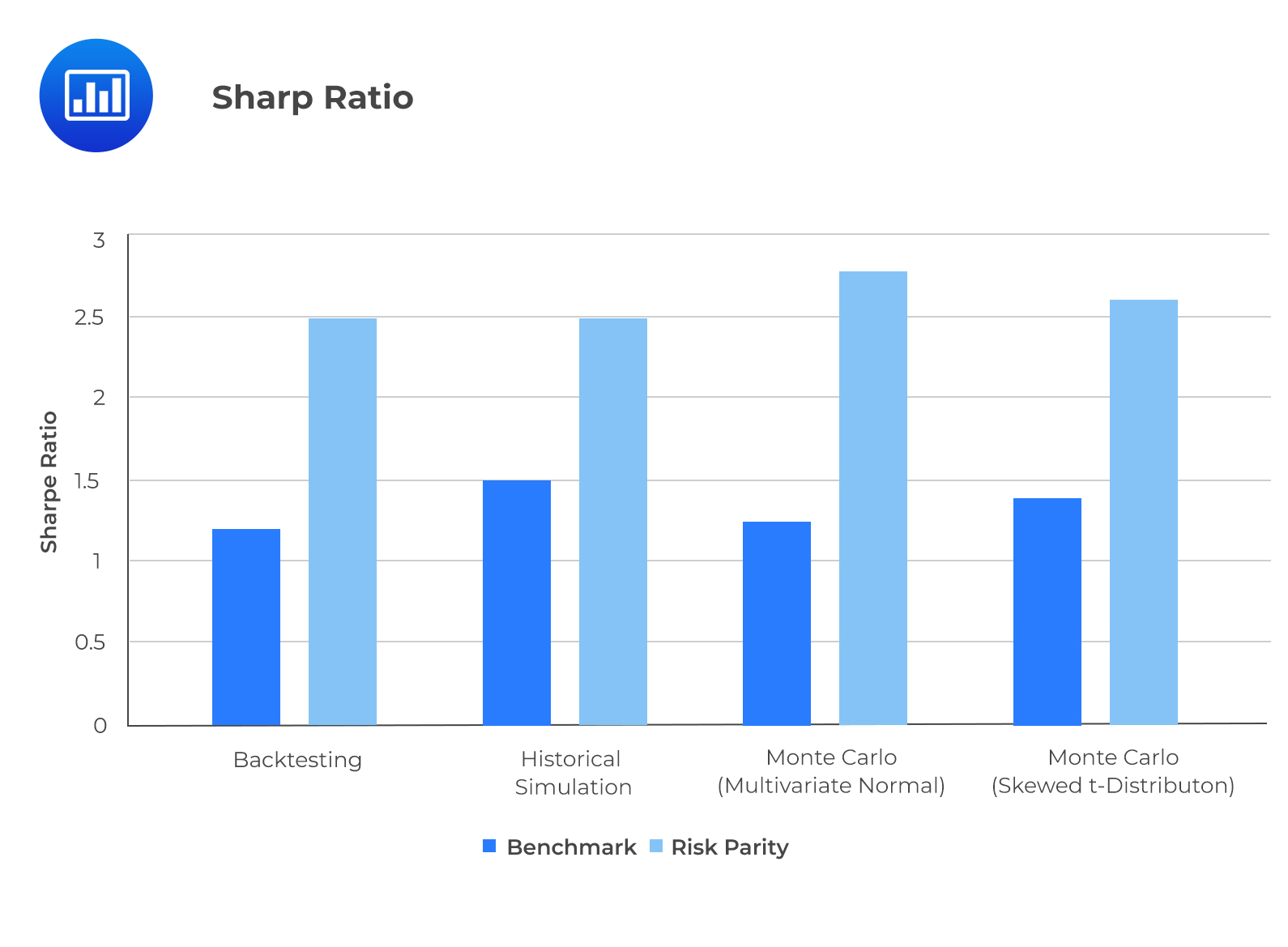
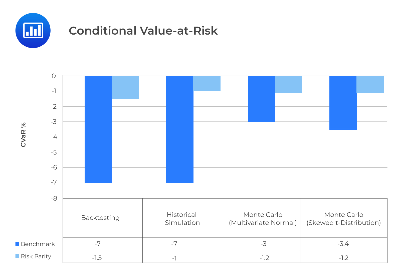
From the following graphs, we can see that the Sharpe ratio is insensitive to all the simulation methods used and maintains that the risk parity strategy outperforms the benchmark strategy. The downside risk (CVaR), on the other hand, is sensitive to the simulation method. The BM strategy results for backtesting and historical simulation are very close. Remember that the multivariate skewed t-distribution and multivariate normal Monte Carlo simulations are very similar. They both underestimate the downside risk of the BM strategy. This is what informs the need for additional sensitivity analysis. The estimated probability density indicates a large difference between the two Monte Carlo simulations and Historical simulation for the BM strategy. The excess kurtosis and negative skewness of the BM strategy’s return explain why the two Monte Carlo simulations fail to account for the left-tail risk parity.

Question

Which of the following situations concerning simulation analysis of a multifactor asset allocation strategy is not likely to involve sensitivity analysis?

1. Changing the specified multivariate normal distribution to a skewed t-distribution.
2. Splitting the rolling window between high-volatility periods and low-volatility periods.
3. Repeating the simulation process with the multivariate skewed t-distribution.

Solution

The correct answer is B.

Splitting the rolling window between high-volatility and low-volatility periods is part of the backtesting simulation.

A and C are incorrect. Both are unique steps in a sensitivity analysis.

Reading 42: Backtesting and Simulation

LOS 42 (h) Demonstrate the use of sensitivity analysis.