General Cash Flows, Portfolios, and Asset Liability Management

After completing this chapter, the candidate will be able to:

1. Define and recognize the definitions of the following terms: yield rate/rate of return, current value, duration and convexity (Macaulay and modified), portfolio, spot rate, forward rate, yield curve, cash flow and duration matching, and immunization (including full immunization and Redington immunization).
2. Calculate:
   • The duration and convexity of a set of cash flows.
   • Either Macaulay or modified duration, given the other.
   • The approximate change in present value due to a change in interest rate, 
     • Using 1^st-order linear approximation based on modified duration.
     • Using 1^st-order linear approximation based on Macaulay duration.
   • The present value of a set of cash flows, using a yield curve developed from forward and spot rates.
3. Construct an investment portfolio to:
   • Protect the value of an asset-liability portfolio using either Redington or full immunization.
   • Exactly match a set of liability cash flows.

Yield Rate

An interest is referred to as a yield rate or the internal rate of return (IRR) if it gives the return an investor can earn from an investment. In other words, it equates the present value of cash inflows to zero.

Assume a project which exists for n years has future cashflows denoted by \( C_1,{C}_2,\ldots,{C}_n \) and denote IRR by i then we have:

$$ \sum_{k=1}^{n}{C_k\left(1+i\right)^{-k}}=\sum_{k=1}^{n}{C_kv^{-k}}=0 $$

This equation can also be written as:

$$ C_0=-\sum_{k=1}^{n}{C_kv^{-k}} $$

This implies that the net present value of the future cash inflows evaluated at a yield rate is equal to the initial cash outlay.

Example: Yield Rate

A project requires a startup of $2,000. It is expected that the investment will earn $800 at the end of the first year and $1,600 after 2 years at will end its transactions. Calculate the internal rate of return of the project.

Solution

We know that

$$ \begin{align*} \sum_{k=1}^{n}{C_kv^{-k}}&=0 \\ \Rightarrow-2000+800v+1600v^2&=0 \\ =4v^2+2v-5&=0 \end{align*} $$

Use the Quadratic formula:

$$ \begin{align*} x&=\frac{-b\pm\sqrt{b^2-4ac}}{2a}. \text{ Where } a=4, b=2, c=-5 \text{ and } x=v \\ \Rightarrow v&=\frac{-2\pm\sqrt{4+80}}{8}=-1.3956 \text{ or } 0.89564 \\ \therefore v&=0.89564\Rightarrow\left(1+i\right)^{-1}=0.895664 \end{align*} $$

So,

$$ i=\left(0.895664 \right)^{-1}-1=0.1165=11.65\% $$

The above example is a case where the equation of value can be solved directly using common mathematical principles to find the yield rate. There is a case where there are more than two cash flows.

It is worth noting that IRR is used in project appraisal. For instance, if the IRR is the same as the effective rate at which bank transaction is done, then the investment is favorable.

The Yield Curve

The interest rate that applies to most investments varies with the term (time) of the investment. This phenomenon is termed as the term structure of interest rates. In other words, rates of interest differ according to the time period of the term of investment, which is, in general, \(i_s\neq i_t\) for all \(s\neq t\), this phenomenon is called the term structure of interest rates, and its corresponding graph of spot rates is called the yield curve.

Yield curves are generally increasing and concave down. If all spot rates are equal, then the yield curve is flat. Until now, the whole course has assumed a flat yield curve (which we have been assuming all along). Conversely, if long-term rates are less than short-term rates, then the yield curve is inverted.

Spot Rates and Forward Rates

Spot Rates

Spot rate can be defined as the annual effective interest earned by funds invested now for a period of time. As such, for t>0 define the spot rate by \( s_t\). Consider the following table

$$ \begin{array}{c|c} \textbf{Length of Investment} & \textbf{Interest Rate} \\ \hline \text{1 year} & {7.00\%} \\ \hline \text{2 years} & {8.00\%} \\ \hline \text{3 years} & {8.75\%} \\ \hline \text{4 years} & {9.25\%} \\ \hline \text{5 years} & {9.50\%} \end{array} $$

All rates shown are annual effective interest rates. Today’s rates, as shown in the table, are called spot rates. Therefore,

$$ s_1=7\%, s_2=8\% \cdots $$

Consider the following timeline:

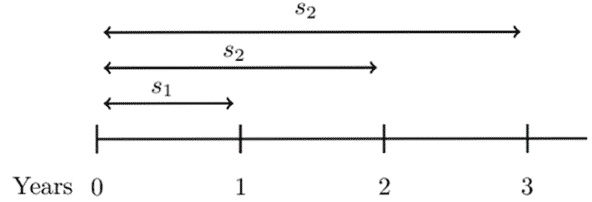
From the timeline, it is easy to see that:

$$ aaf_0^1=1+s_1\Rightarrow adf_1^0=\left(1+s_1\right)^{-1}= v_1 \\ paf_0^2=\left(1+s_2\right)^2\Rightarrow ppf_2^0=\left(1+s_2\right)^{-2}=v_2^2 \\ ppf_0^3=\left(1+s_3\right)^3\Rightarrow ppf_3^0=\left(1+s_3\right)^{-3}=v_3^3 $$

Note that aaf = annual accumulation factor, adf= annual discount factor, paf= periodic accumulation factor and pdf= periodic discount factor.

Forward Rates

A forward rate is an effective rate of interest that is applicable to financial transactions that will take place in the future. We can relate the spot rates and forward rates.

Consider the following timeline:

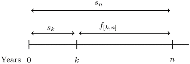
\( f_{\left[k,n\right]} \) denotes the forward rate from time k to time n, and it is the annual effective interest rate used to accumulate or discount between times k and n.

It is easy to note that,

$$ \begin{align*} aaf_0^n&=aaf_0^k\cdot aaf_k^n \\ \Rightarrow\left(1+s_n\right)^n&=\left(1+s_k\right)^k.\left(1+f_{\left[k,n\right]}\right)^{n-k} \\ \therefore\left(1+f_{\left[k,n\right]}\right)^{n-k}&=\frac{\left(1+s_n\right)^n}{\left(1+s_k\right)^k} \end{align*} $$

Example: Spot Rates and Forward Rates

Consider the following annual effective rates (spot rates).

$$ \begin{array}{c|c} \textbf{Length of Investment} & \textbf{Interest Rate} \\ \hline \text{1 year} & {7.00\%} \\ \hline \text{2 years} & {8.00\%} \\ \hline \text{3 years} & {8.75\%} \\ \hline \text{4 years} & {9.25\%} \\ \hline \text{5 years} & {9.50\%} \end{array} $$

Determine the forward rate from year 2 to year 3.

Solution

Consider the following timeline:

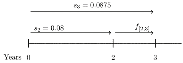
So,

$$ \begin{align*} \left(1+s_3\right)^3&=\left(1+s_2\right)^2\cdot1+f[2,3] \\ \Rightarrow\left(1.0875\right)^3&=\left(1.08\right)^2\cdot\left(1+f_{\left[2,3\right]}\right)\\ \therefore f_{\left[2,3\right]}&=\frac{\left(1.0875\right)^3}{\left(1.08\right)^2}=0.10265=10.3\% \end{align*} $$

Alternatively, we can use the formula above so that:

$$ \begin{align*} \left(1+f_{\left[2,3\right]}\right)^{3-2}&=\frac{\left(1+s_3\right)^3}{\left(1+s_2\right)^2}\\ \Rightarrow1+f_{\left[2,3\right]}&=\frac{\left(1.0875\right)^3}{\left(1.08\right)^2}=1.1027 \\ \therefore f_{\left[2,3\right]}&=0.10265=10.3\% \end{align*} $$

Spot Rates, Forward Rates, and Zero-Coupon Bonds

Spot rates are mostly based on zero-coupon bonds. As such, spot rates are also termed as zero-coupon rates. Assume a zero-coupon bond of the term \( \textbf{n} \) (say) with an issue price, \( \textbf{P}_\textbf{n} \).

Discrete-time Spot Rates

The yield on a unit zero-coupon bond is called n-year spot rate of interest denoted by \( s_n \). It is the measure of the mean interest rate from now until the end of n- years. The equation of value of a unit zero-coupon bond will be:

$$ P_n=\left(1+s_n\right)^{-n}\Rightarrow\left(1+s_n\right)=P_n^{-\frac{1}{n}} $$

Also, note that:

$$ \left(1+s_n\right)^n=v^{-n} $$

Example: Discrete-time Spot Rate

Calculate the one-year spot rate of a zero-coupon bond priced at $94 per $100 nominal.

Solution

$$ P_n=\left(1+s_n\right)^{-n} \\ \Rightarrow100\left(1+s_n\right)^{-1}=94\therefore s_n=\left(\frac{94}{100}\right)^{-1}=0.06382=6.82% $$

The yield curve can also represent the redemption yields meaning it is not necessarily the spot rates.

Discrete-time Forward Rates

The discrete forward which can be denoted by \( f_{\left[k,n\right]} \) is the yearly rate of interest, which is agreed upon at time 0 for an investment made at time k>0 for a period of n-k years.

For example, an investor agrees to invest $50 at time k for n-k years, then the accumulated amount at time n is:

$$ 50(1+f_{\left[k,n\right]}) $$

Briefly, the forward rate of interest \( f_{k,n} \) measures the mean interest rate between times k and n.

There is, however, a connection between the spot rates and forward rates. The accumulation amount at time k of investment of 1 at time t=0 is given by \( \left(1+s_k\right)^k\). If we had agreed to invest this amount at time k for n-k years so that the accumulation at time n will be:

$$ \left(1+s_k\right)^k.\left(1+f_{\left[k,n\right]} \right) $$

We are also aware that 1 invested at time 0 for n years will be

$$ \left(1+s_n\right)^n $$

Note also that the price of a zero-coupon bond of 1 invested for n years accumulates to \( P_n^{-n} \)

$$ \Rightarrow\left(1+s_k\right)^k.\left(1+f_{\left[k,n\right]} \right)=\left(1+s_n\right)^n=P_n^{-n} $$

From this, we get the following relationship:

$$ \left(1+f_{\left[k,n\right]}\right)^{n-k}=\frac{\left(1+s_n\right)^n}{\left(1+s_k\right)^k}=\frac{P_k}{P_n} $$

From these relationships, it is clear that the full-term structure of interest rates may be determined by the given spot rates and forward rates.

For a one-period rate, \( f_k=f_{k,1} \). Also, define \(f_0=s_1\) . Using the same arguments,

$$ \Rightarrow\left(1+s_n\right)^n=\left(1+f_0\right)\left(1+f_1\right)\left(1+f_2\right)\ldots(1+f_{n-1}) $$

The one-year forward rate \( f_t=f_{t,1} \) is the rate in the time interval (k,k+1) and can represented as:

$$ 1+f_t=\frac{\left(1+s_{k+1}\right)^{k+1}}{\left(1+s_k\right)^k} $$

Example: Forward Rates

Given that 6%, 5.7%, and 5% are the 3, 5, and 7-year spot rates per year, respectively, and that the forward rate from time 4 is 5.2% per year, find f[5,7]

Solution

We are given \(s_3=6\%, s_5=5.7\% s_7=5\%, f[3,7]=5.2\% \)

We know that

$$ \begin{align*} \left(1+f_{\left[k,n\right]} \right)^{n-k}&=\frac{\left(1+s_n\right)^n}{\left(1+s_k\right)^k}=\frac{P_k}{P_n} \\ \Rightarrow \left(1+f_{\left[5,7\right]} \right)^{(7-5)}&=\frac{\left(1+s_7\right)^7}{\left(1+s_5\right)^5} \\\Rightarrow \left(1+f_{\left[5,7\right]}\right)^2&=\frac{\left(1.05\right)^7}{\left(1.057\right)^5}\\\Rightarrow f_{\left[5,7\right]}&=\left[\frac{\left(1.05\right)^7}{\left(1.057\right)^5}\right]^{\frac{1}{2}}-1=3.27\% \end{align*} $$

Example: Spot Rates, Forward Rates, and Zero-Coupon Bonds

You are given the following prices for 1000 par value zero-coupon bonds:

$$ \begin{array}{c|c} \textbf{Duration} & \textbf{Price} \\ \hline \text{1 year} & {970} \\ \hline \text{2 years} & {940} \\ \hline \text{3 years} & {910} \end{array} $$

Determine the forward rate from time 2 to time 3 that corresponds to these prices.

Solution

Consider the following timeline:

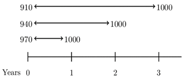
We know that,

$$ \begin{align*} \left(1+f_{\left[k,n\right]} \right)^{n-k}&=\frac{\left(1+s_n\right)^n}{\left(1+s_k\right)^k}=\frac{P_k}{P_n} \\ \Rightarrow \left( 1+f[2,3] \right)&=\frac{\left(1+s_3\right)^3}{\left(1+s_2\right)^2}=\frac{P_2}{P_3}=\frac{940}{910} \\ \Rightarrow f[2,3]&=\frac{94}{91}-1=0.03296=3.30\% \end{align*} $$

Alternatively, we can use the fact that:

$$ \left(1+s_n\right)^n=v^{-n} $$

Consider the following timeline:

It is easy to see that:

$$ \left(1+s_3\right)^3=\left(1+s_2\right)^2\cdot\left(1+f[2,3]\right) \\ v_3^{-3}=v_2^{-2}\cdot1+f[2,3] $$

From the tables, we know that,

$$ 940=1000v_2^2\Rightarrow v_2^2=0.94 $$

And,

$$ \begin{align*} 910&=1000v_3^3\Rightarrow v_3^3=0.910 \\ \Rightarrow{0.91}^{-1}&={0.94}^{-1}\cdot\left(1+f_{\left[2,3\right]}\right)\Rightarrow f_{\left[2,3\right]}=\frac{94}{91}-1=0.03296=3.30\% \end{align*} $$

Example: Implied Yield on Coupon Bonds

You are given that the annual yield on zero-coupon bonds with a duration of k years is \(i_k\)=0.03+0.005(k-1).

Determine the annual yield rate for a 3-year bond with 5% annual coupons that are consistent with this term structure of interest rates.

Solution

From the annual yield function, we have that:

$$ s_1=i_1=0.030, s_2=i_2=0.035 \text{ and } s_3=i_3=0.040 $$

Now, consider the following timeline:

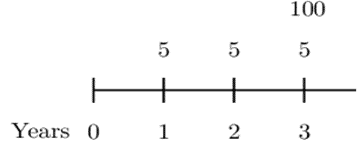
Then the equation of value is:

$$ \begin{align*} 5\cdot v_1&+5\cdot v_2^2+105v_3^3=5\cdot a_{\overline{3}|i}+100v_i^3 \\ \Rightarrow\frac{5}{1.03}&+\frac{5}{{(1.035)}^2}+\frac{105}{{(1.04)}^3}=5\cdot a_{\overline{3}|i}+100v_i^3 \\ \therefore5\cdot a_{\overline{3}|i}&+100v_i^3=102.866\Rightarrow i=0.03967=3.97\% \end{align*} $$

Therefore, the yield curve defined by the \( i_k=0.03+0.005(k-1) \) on a 3-year bond implies an annual rate of 3.97%.

Continuous-time Spot Rates

The continuous-time spot rate is defined as the force of interest that is equivalent to an effective rate of interest rate, which corresponds to the spot rate. Like in discrete-time spot rate, let \( P_n \) be the price of a unit zero-coupon bond with the term n-years. Then,

$$ P_n=e^{-\left(\delta_nn\right)}\Rightarrow\delta_n=-\frac{1}{n}\ln{P_n} $$

Where \( \delta_n \) is the n-year spot force of interest. It is also called the continuously compounded spot rate of interest or the continuous-time spot rate.

The n-year spot force of interest is connected to the corresponding discrete-time spot rate \(s_n\) just like i and \(\delta\) that is,1+i= \(e^\delta\). Similarly to spot rates,

$$ 1+s_n=e^{\delta_n}\Rightarrow s_n=e^{\delta_n}-1 $$

Continuous-time Forward Rates

Denote continuous-time forward rate of interest from time k to n by \(F_{[k,n]}\). It is defined as the force of interest equivalent to the annual forward interest \(f_{[k,n]}\). If $1 is invested for n-k years starting at time k which is agreed at time \( 0 \le k \) accumulates to \( \left(1+f_{\left[k,n\right]}\right)^{n-k} \) at time n using the annual forward rates \(f_{\left[k,n\right]}\). Now, applying the equivalent forward force of interest, the same investment will accumulate to

$$ e^{(n-k)F[k,n]} $$

Therefore, the relationship is given by:

$$ f_{[k,n]}=e^{(n-k)F[k,n]}-1 $$

Now consider the investment of $1 at time 0 using the spot rate \(\delta_k\) for k years and then followed by forward rates \(F[k,n]\). This is similar to the investment of $1 at a continuous-time spot rate \(\delta_n\) for n years. Therefore:

$$ \begin{align*} e^{k\delta_k}e^{(n-k)F_{[k,n]}}]&=enδn\\ \Rightarrow k\delta_k+(n-k)F_{[k,n]}&=nδn\\ \therefore F_{[k,n]}&=\frac{n {\delta_n}-k {\delta_k}}{n-k} \end{align*} $$

Now using the relation \( \delta_n=-\frac{1}{n}\ln{P_{n }} \) then, the above equation reduces to (the algebra is trivial)

$$ \begin{align*} F[k,n]&=\frac{(n)-\frac{1}{n}lnP_n -(k).-\frac{1}{k}lnP_k} {n-k} \\ &=\frac{1}{n-k}\left[\ln{P_k}-\ln{P_n}\right] \\ \therefore F[k,n]&=\frac{1}{n-k}ln\left[\frac{P_k}{P_n}\right] \end{align*} $$

Example: Continuous Forward Rates

The prices for the zero-coupon bonds at various years are as follows:

1 year=94%, 5 years=70%, 10 years=47%, 15 years=30%.

Calculate the continuous-time forward rates between year 5 and year 15.

Solution

We know that

$$ \begin{align*} F_{[k,n]}&=\frac{1}{n-k}ln\left[\frac{P_k}{P_n}\right] \\ \Rightarrow F_{[5,15]}&=\frac{1}{10}ln(\frac{P5}{P15})=\frac{1}{10}ln(\frac{70}{30})=0.08473=8.473\% \end{align*} $$

Duration and Convexity

Duration and convexity are the simplest measures of the vulnerability of a portfolio to interest rate risk, where interest rate risk is the risk that arises from fluctuating interest rates. These measures assume a flat yield curve, which means that when the rates change, all other changes are equal.

Suppose that an institution has discounted assets of value V (A), which is supposed to meet the discounted liabilities V (L). If the interest rises, then both will decrease and vice versa. In order to examine these changes as the interest rates change, we use the changes in yield to maturity to represent changes in the underlying term structure.

Modified Duration

Modified duration expresses the change in the value of an asset or portfolio in response to a change in interest rates. Consider a series of cash flows of a portfolio \( C_t \) for all \( t=1,2,\ldots,n\). Let \(P\) be the present values of the payments at rate \(i\) (yield to maturity). Therefore:

$$ P(i)=\sum_{t=1}^{n}{C_tv^t } $$

The modified duration is defined to be:

$$ \begin{align*} \text{ModD}&=-\frac{1}{P(i)}\frac{dP(i)}{di}=-\frac{P^\prime(i)}{P(i)}\\ &=\left(\frac{1}{\sum_{t=1}^{n}{C_tv^t }}\right)\left(\sum_{k=1}^{n}{t.C_tv^{t+1}}\right)=\frac{\sum_{k=1}^{n}{t.C_tv^{t+1}}}{\sum_{t=1}^{n}{C_tv^t }} \end{align*} $$

It is important to note that the differentiation is done with respect to \(i\) and not \(v\) that is, if

$$ \begin{align*} P(i)&=\sum_{t=1}^{n}{{t\cdot C}_tv^t }=\sum_{k=1}^{n}{C_t{(1+i)}^{-t}\Rightarrow\frac{dP(i)}{di}=\sum_{k=1}^{n}{(-t)C_t\left(1+i\right)^{-t-1} }} \\ &=(-1)\sum_{k=1}^{n}{t.C_tv^{t+1} } \\ \Rightarrow-\frac{1}{P\left(i\right)}\frac{dP\left(i\right)}{di}&=-\frac{\left(-1\right)\sum_{k=1}^{n}{t.C_tv^{t+1}}}{\sum_{t=1}^{n}{C_tv^t}}=\frac{\sum_{k=1}^{n}{t.C_tv^{t+1}}}{\sum_{t=1}^{n}{C_tv^t }} \end{align*} $$

Modified duration is always positive, and it measures the percentage decrease of the value of the investment per unit increase in the yield to maturity.

Macaulay Duration

Just as modified duration, Macaulay duration is also a measure of portfolio sensitivity to the interest rate. Macaulay duration is defined as the average of the term of cash flows \( (C_t) \) weighted by the present value and expressed as the number of payments periods. In other words, the Macaulay duration of a set of payments is the weighted average of the times of the payments, where the weight of the payment at time \(t\) is equal to the present value of the payment at time t divided by the present value of all the payments. 

Consider the following timeline:

By definition,

$$ \begin{align*} \text{MacD}&=\frac{1\cdot C_1\cdot v+{2\cdot C}_2\cdot v^2+{3\cdot C}_3\cdot v^3+\cdots}{C_1\cdot v+C_2\cdot v^2+C_3\cdot v^3+\cdots}\\ &=\frac{\sum{{t\cdot C}_tv^t}}{\sum{C_t\cdot v^t}} \end{align*} $$

Note that factoring out \((1+i)\) in the numerator of the above equation then:

$$ \begin{align*} \text{MacD}&=\frac{(1+i)\sum_{t=1}^{n}{tC_tv^{t+1} }}{\sum_{t=1}^{n}{C_tv^t }}=\left(1+i\right) \text{ModD} \\ \Rightarrow \text{MacD}&=\text{ModD}\left(1+i\right)\Longleftrightarrow \text{ModD}=\text{MacD}\cdot v \end{align*} $$

The Macaulay duration of a bond that pays an annual coupon of \(D\) and redeemed at \(R\) is given by:

$$ \text{MacD}=\frac{D\left(Ia\right)_{\overline{n|}}+Rnv^n}{Da_{\overline{n|}}+Rv^n} $$

If it is a zero-coupon bond of the nominal amount of $100 then,

$$ \text{MacD}=\frac{100nv^n}{100v^n}=n $$

This is obvious since the mean term of equal payments must be the time of that cash flow.

Example: Macaulay Duration

Calculate the Macaulay Duration of a bond redeemable at par in 10 years that has an annual coupon of 8% and an interest rate of 10% per annum.

Solution

$$ \begin{align*} \text{MacD}&=\frac{D\left(Ia\right)_{\overline{n|}}+Rnv^n}{Da_{\overline{n|}}+Rv^n} \\ &=\frac{8\left(Ia\right)_{\overline{10|}}+10\times100v^{10}}{8a_{\overline{10|}}+100v^{10}}=\frac{617.83}{87.71}=7.04 \text{ years} \end{align*} $$

Duration of a Portfolio of Assets

The duration of a portfolio of assets equals the weighted average of the duration of the assets that form the portfolio, with the weight associated with the duration of an individual asset being the ratio of the price of that asset to the price of the portfolio.

Consider a portfolio with three assets A, B, and C. Then,

$$ \begin{align*} \text{MacD}_{pf}&=\frac{\left(\sum{{t\cdot C}_t\cdot v^t}\right)_{Pf}}{\left(\sum{C_t\cdot v^t}\right)_{Pf}}\\ &=\frac{\left(\sum{{t\cdot C}_t\cdot v^t}\right)_A+\left(\sum{{t\cdot C}_t\cdot v^t}\right)_B+\left(\sum{{t\cdot C}_t\cdot v^t}\right)_C}{P_{Pf}}\\ &=\frac{\left(\sum{{t\cdot C}_t\cdot v^t}\right)_A}{P_{Pf}}+\frac{\left(\sum{{t\cdot C}_t\cdot v^t}\right)_B}{P_{Pf}}+\frac{\left(\sum{{t\cdot C}_t\cdot v^t}\right)_C}{P_{Pf}}\\ &=\frac{P_A}{P_{Pf}}\cdot\frac{\left(\sum{{t\cdot C}_t\cdot v^t}\right)_A}{P_A}+\frac{P_B}{P_{Pf}}\cdot\frac{\left(\sum{{t\cdot C}_t\cdot v^t}\right)_B}{P_B}+\frac{P_C}{P_{Pf}}\cdot\frac{\left(\sum{{t\cdot C}_t\cdot v^t}\right)_C}{P_C}\\ &=\frac{P_A}{P_{Pf}}\cdot\left(MacD\right)_A+\frac{P_B}{P_{Pf}}\cdot\left(MacD\right)_B+\frac{P_C}{P_{Pf}}\cdot\left(MacD\right)_C \end{align*} $$

Note that

$$ P_{Pf}=P_A+P_B+P_C $$

Example: Duration of a Portfolio of Assets

A portfolio of assets has three types of bonds with the following characteristics:

Bond A has a price of 2,000 and a Macaulay duration of 9.5

Bond B has a price of 3,000 and a Macaulay duration of 9.0

Bond C has a price of 5,000 and a Macaulay duration of 16.0

All prices and Macaulay durations above were calculated using an annual effective interest rate of 6%.

Determine the Macaulay duration of the portfolio using an annual effective interest rate of 6%.

Solution

We have:

$$ \begin{align*} P_{Pf}&=P_A+P_B+P_C \\ &=2000+3000+5000 \\ &=10000 \end{align*} $$

Then,

$$ \text{MacD}_{pf}=\frac{2000}{10000}\left(9.5\right)+\frac{3000}{10000}\left(9.0\right)+\frac{5000}{10000}\left(16.0\right)=12.6 $$

Convexity

Convexity is a measure of the curvature in the relationship between the price and yield of a bond. Whereas duration is the first derivative of the price of the bond with respect to interest rates, convexity is the second derivative of the price of the bond with respect to interest rates. Graphically, it can be represented as follow:

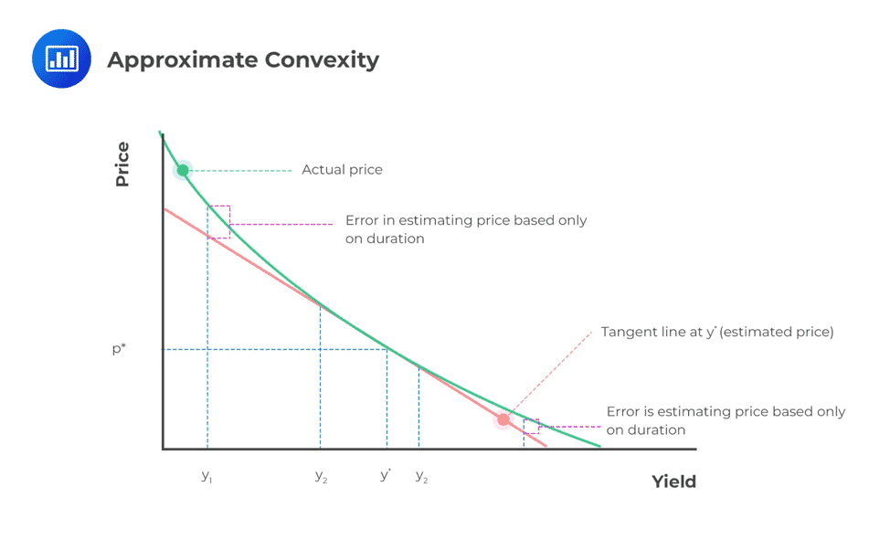Convexity determines precisely the effect of interest changes on a portfolio by giving a measure of the change in the duration of a bond when the interest rate changes. It implies that (\P\) increases when there is a decrease in the interest rate and increases when there is the same level in the interest rate.

Definition: The Macaulay convexity of a set of payments is the weighted average of the squares of the times of the payments, where the weight assigned to the payment at time t is equal to the present value of the payment at time t divided by the present value of all the payments. Macaulay convexity is defined as:

$$ MacC=\frac{1^2\cdot C_1\cdot v+{2^2\cdot C}_2\cdot v^2+{3^2\cdot C}_3\cdot v^3+\cdots}{C_1\cdot v+C_2\cdot v^2+C_3\cdot v^3+\cdots}=\frac{\sum{{t^2\cdot C}_t\cdot v^t}}{\sum{C_t\cdot v^t}} $$

On the other hand, modified convexity is defined as:

$$ \begin{align*} \text{ModC}&=\frac{1}{P}\frac{d^2}{di^2}P=\frac{P^{\prime\prime}(i)}{P(i)}\\ &=\left(\frac{1}{\sum{C_t\cdot v^t}}\right)\left(\sum{t\left(t+1\right)C_tv^{t+2}}\right)=\frac{\sum{t\left(t+1\right)C_tv^{t+2}}}{\sum{C_t\cdot v^t}} \end{align*} $$

Convexity is always positive.

Example: Modified and Macaulay Convexities

Consider the following payments presented in the following timeline.

For the set of payments above, using i=0.06, determine

1. the Macaulay convexity, and
2. the modified convexity.

Solution

a)

$$ \begin{align*} \text{MacC}&=\frac{\sum{{t^2\cdot C}_t\cdot v^t}}{\sum{C_t\cdot v^t}}\\ &=\frac{1^2\cdot10\cdot v+2^2\cdot20\cdot v^2+3^2\cdot1030\cdot v^3}{10\cdot v+20\cdot v^2+1030\cdot v^3}\\ &=8.815 \end{align*} $$

b)

$$ \begin{align*} \text{ModC}&=\frac{\sum{t\left(t+1\right)C_tv^{t+2}}}{\sum{C_t\cdot v^t}}\\ &=\frac{20\cdot\left(1+i\right)^{-3}+120\cdot\left(1+i\right)^{-4}+12360\cdot\left(1+i\right)^{-5}}{10\cdot\left(1+i\right)^{-1} +20\cdot\left(1+i\right)^{-2}+1030\cdot\left(1+i\right)^{-3}}\\ &=\frac{9,347.95}{892.04}=10.48 \end{align*} $$

Example: Modified Convexity

An annuity pays $X forever from a lump sum deposited in a bank account for an infinite term that pays a simple interest i, at a constant rate at the end of each year.

Find the expression of modified convexity.

Solution

$$ \begin{align*} P(i)&=Xa_{\overline{\infty|}}=\frac{X}{i} \\ c\left(i\right)&=\frac{1}{P\left(i\right)}\frac{d^2}{di^2}P(i)=\frac{P^{\prime\prime}(i)}{P(i)}=\frac{\frac{2X}{i^3}}{\frac{X}{i}}=\frac{2}{i^2} \end{align*} $$

First Order Approximations

1st Order Linear Approximation Based on Modified Duration

Using modified duration and convexity, we can approximate change in the present value P(i) (which in this case can be a price of a bond) as follows:

Let \( \Delta i=i_{new}-i_{old} \) be the change in the rate of interest. Then using the Taylor series expansion and using modified duration only, then:

$$ \begin{align*} \Rightarrow P\left(i+\Delta i\right)&=P\left(i\right)+\frac{dP\left(i\right)}{di}\epsilon_i \\ &=P\left(i\right)\left[1-\left(-\frac{1}{P\left(i\right)}\frac{dP\left(i\right)}{di}\right)\Delta_i\right] \end{align*} $$

Since,

$$ \begin{align*} \text{ModD}&=-\frac{1}{P(i)}\frac{dP(i)}{di}\\ \Rightarrow P\left(i+\Delta i\right)&=P\left(i\right)\left[1-\text{ModD}.\Delta_i\right] \end{align*} $$

Clearly, the change in price \( \Delta P(i) \) is

$$ \begin{align*} \Delta P\left(i\right)&=-P\left(i\right).\text{ModD}.\Delta_i\\ \Rightarrow P\left(i+\Delta i\right)&=P\left(i\right)-\Delta P\left(i\right) \end{align*} $$

We also know that,

$$ \text{ModD}=\text{MacD}\cdot v $$

Thus, we can write,

$$ \begin{align*} P\left(i+\Delta i\right)&=P\left(i\right)\left[1-ModD.\Delta_i\right]\\ &=P\left(i\right)\left[1-MacD\cdot v.\Delta_i\right]\\ &=P\left(i\right)-P\left(i\right).MacD\cdot v.\Delta_i\\ \Rightarrow\Delta P\left(i\right)&=-P\left(i\right).MacD\cdot v.\Delta_i \end{align*}$$

1st Order Approximation Based on Macaulay Duration

If we use Macaulay duration only, we have:

$$ ∆P(i)=P(i)∙\left[\left( \cfrac{1+i_\text{old}}{1+i_\text{new}}\right)^\text{MacD}-1\right] $$

So,

$$ P\left(i+\Delta i\right)=P\left(i\right)-∆P(i) $$

Note that,

$$ P\left(i\right)=P\left(i_{old}\right) $$

And

$$ \Delta i=i_\text{new}-i_\text{old} $$

Example: First Order Approximations based on Modified and Macaulay Durations

A bond has a price of 7025 to yield 7% annual effective. Using this same yield rate, the Macaulay duration of the bond is 4.95 years. Determine the price of the bond to yield 6.5% annual effective, using

1. the first-order modified approximation, and
2. the first-order Macaulay approximation.

Solution

1. Since we are given Macaulay duration, we have

   $$ \begin{align*} P\left(i+\Delta i\right)&=P\left(i\right)\left[1-\text{ModD}.\Delta_i\right]\\ &=P\left(i\right)\left[1-\text{MacD}\cdot v.\Delta_i\right] \\ &=P\left(i\right)-P\left(i\right).\text{MacD}\cdot v.\Delta_i \\ P\left(0.065\right)&=P\left(0.07\right)-P\left(0.07\right).\frac{4.95}{1.07}. (0.07-0.065)\\ &=7025-7025\cdot\frac{4.95}{1.07}\cdot(0.065-0.07) \\ &=7025+162=7187 \end{align*} $$

2. Macaulay duration first approximation is given:

   $$ \begin{align*} \Delta P&=P(i).\left[\left( \cfrac{1+i_{old}}{1+i_{new}}\right)^ \text{MacD}-1 \right] \\ &=7025\cdot\left[\left(\frac{1.07}{1.065}\right)^{4.95}-1\right]=165 \\ \Rightarrow P\left(0.065\right)&=7025+165=7190 \end{align*} $$

Calculating Either Macaulay or Modified Duration Given the Other

Consider an n-year annual coupon bond, redeemable at par, and bought to yield an annual effective interest rate that is equal to the coupon rate as shown by the following timeline,

The Macaulay and modified durations can be shown to be:

$$ \text{MacD}={\ddot{a}}_{\overline{n}|} $$

And

$$ \text{[ModD}=\text{MacD} \cdot v=a_{\overline{n}|} $$

Similarly, consider an n-year monthly coupon bond, redeemable at par, is bought to yield a monthly effective interest rate that is equal to the monthly effective coupon rate,

The Macaulay and modified durations are given by:

$$ \text{MacD}={\ddot{a}}_{\overline{12n}|} $$

And

$$ \text{ModD}= \text{MacD} \cdot v=a_{\overline{12n}|} $$

Consider the following example:

Example: Calculating Either Macaulay or Modified Duration Given the Other

A 20-year annual coupon bond, redeemable at par, is bought to yield an annual effective interest rate that is equal to the coupon rate.

Determine an expression for the Macaulay duration of the bond.

Solution

We know that:

$$ \text{MacD}=\frac{\sum{{t\cdot C}_tv^t}}{\sum{C_t\cdot v^t}} $$

So, in this case, we have,

$$ \begin{align*} \text{MacD} &=\frac{1\cdot F r\cdot v+2\cdot F r\cdot v^2+\ldots+20\cdot F r\cdot v^{20}+20\cdot F\cdot v^{20}}{Fr\cdot a_{\overline{20}|}+F\cdot v^{20}}\\ &=\frac{Fr\cdot\left(Ia\right)_{\overline{20}|}+20\cdot F\cdot v^{20}}{Fr\cdot a_{\overline{20}|}+F\cdot v^{20}}\\ &=\frac{r\cdot\left(Ia\right)_{\overline{20}|}+20\cdot v^{20}}{r\cdot a_{\overline{20}|}+v^{20}}\\ &=\frac{r\cdot\left[\frac{{\ddot{a}}_{\overline{20}|}-20v^{20}}{i}\right]+20\cdot v^{20}}{r\cdot\left[\frac{1-v^{20}}{i}\right]+v^{20}} \end{align*} $$

Now since, i=r, we have

$$ \text{MacD}=\frac{r\cdot\left[\frac{{\ddot{a}}_{\overline{20}|}-20v^{20}}{i}\right]+20\cdot v^{20}}{r\cdot\left[\frac{1-v^{20}}{i}\right]+v^{20}}=\frac{{\ddot{a}}_{\overline{20}|}-20v^{20}+20\cdot v^{20}}{1-v^{20}+v^{20}}={\ddot{a}}_{\overline{20}|} $$

Which proves our result. Also, note that,

$$ \text{ModD}=\text{MacD}\cdot v=v.{\ddot{a}}_{\overline{20}|}=a_{\overline{20}|} $$

Exact Matching (Dedication)

Suppose that an organization, at a valuation interest \(i\), has a present value of liabilities \(P_L\left(i\right)\) and the present value of the assets \(P_A\left(i\right)\). If it were possible to select a portfolio of assets that generates cash flows that exactly match the liabilities of the fund in terms of timing and amount, then the fund would be completely insulated against fluctuations of the interest rates. This is called an exact matching or dedication. Exact matching is just a theoretical concept, and in most cases, not achievable.

Example: Exact Matching (Dedication)

A company has a 95,030 liability due in one year and another 297,330 liability due in two years. The company has the following two types of bonds they can use to match these liabilities exactly:

• Bond A is a two-year 1000 par value bond with 6% annual coupons.
• Bond B is a one-year zero-coupon bond redeemable at 1000.

Determine the number of each type of bond the company should buy in order to exactly match the liabilities.

Solution

Let n be the number of bonds of type Bond A purchased.

Let m be the number of bonds of type Bond B purchased.

Consider the following timeline:

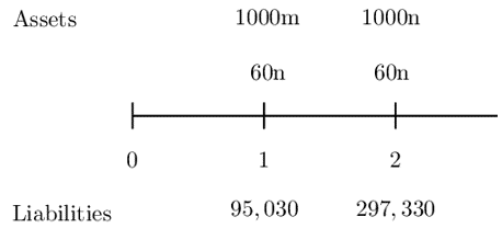
From the timeline,

• Bond A: two-year 1000 par value with 6% annual coupons (n of these).
• Bond B: one-year zero-coupon bond redeemable at 1000 (m of these).

Therefore the equations of values are given by:

$$ \begin{align*} 1000m+60n&=95,030\ldots\ldots\ldots(i) \\ 1060n&=297,330\ldots\ldots\ldots(ii) \end{align*} $$

Substituting Eq (ii) in Eq (i) we have:

$$ n=280.5\quad \& \quad m=78.2 $$

Immunization

It is possible to choose an asset portfolio that offers considerable protection against small changes in interest rates. Now, define the net present value function as:

$$ P\left(i\right)=P_A\left(i\right)-P_L\left(i\right) $$

The idea behind the immunization is that, given a specific interest rate, \(i=i_0\), if possible, we have assets and liabilities arranged so that the graph of \(y=P(i)\) has a minimum of 0 located at \(i=i_0\).

In simple terms, immunization is the process of selecting asset portfolios that will protect the net present value function against small interest rate fluctuations.

Conditions Required for Immunizations

Condition 1

The first condition requires that the net present value function is equal to zero. That is:

$$ P\left(i\right)=P_A\left(i\right)-P_L\left(i\right)=0 $$

It, therefore, implies that:

$$ P_A\left(i\right)=P_L\left(i\right) $$

Condition 2

The second condition requires that the first derivative of the net present value function be equal to 0. That is:

$$ P^{\prime}\left(i_0\right)=0 $$

From the first condition, it is easy to see that:

$$ P_A^{\prime}\left(i_0\right)=P_L^{\prime}\left(i_0\right) $$

Recall that we defined a modified duration as:

$$ ModD=\frac{-P^{\prime}(i)}{P(i)} $$

Using the first and the second conditions, we have the that:

$$ {ModD}_A\left(i_0\right)={ModD}_L\left(i_0\right) $$

Note that this is also true for Macaulay’s duration:

$$ {MacD}_A\left(i_0\right)={MacD}_L\left(i_0\right) $$

Condition 3

In order to make sure that the net present value function has a minimum of 0 located at \(i=i_0\), then the second derivative of the net present value function should be positive so that the graph is concave up. That is:

$$ P^{\prime\prime}\left(i_0\right)>0 $$

Now we know that:

$$ P\left(i\right)=P_A\left(i\right)-P_L\left(i\right) $$

Since the derivative is a linear operator, we have that:

$$ \begin{align*} P^{\prime\prime}\left(i_0\right)&=P_A^{\prime\prime}i-P_L^{\prime\prime}i>0 \\ \Rightarrow& P_A^{\prime\prime}\left(i_0\right)> P_L^{\prime\prime}\left(i_0\right) \end{align*} $$

Recall that modified convexity is defined as:

$$ ModC=\frac{P^{\prime\prime}(i)}{P(i)} $$

Now using condition 1 and condition 3, it is easy to see that:

$$ {ModC}_A\left(i_0\right)>{ModC}_L\left(i_0\right) $$

Note that this is also true for the Macaulay convexity. That is:

$$ {MacC}_A\left(i_0\right)>{MacC}_L\left(i_0\right) $$

The conditions discussed above are called Redington’s Immunization, named after a British actuary Frank Redington. Briefly, Redington’s condition can be stated as:

1. The present value of the assets equals the present value of the liabilities. That is, $$ P_A\left(i\right)=P_L\left(i\right) $$
2. The duration of the assets equals the duration of the liabilities.

   $$ {ModD}_A\left(i_0\right)={ModD}_L\left(i_0\right) $$

   And

   $$ {MacD}_A\left(i_0\right)={MacD}_L\left(i_0\right) $$

3. The convexity of the assets is greater than the convexity of the liabilities. That is:

   $$ {ModC}_A\left(i_0\right)>{ModC}_L\left(i_0\right) $$

   And

   $$ {MacC}_A\left(i_0\right)>{MacC}_L\left(i_0\right) $$

Example: Redington Immunization Conditions

A company has to pay $2000 at the end of 2 years and $4000 after 4 years. The present annual effective rate of interest is 10%. The company wishes to immunize the interest rate risk by investing in zero-coupon bonds. A risk manager advises the company to buy the following zero-coupon bonds:

• One-year zero-coupon bond with a face value of $44.74
• Three-year zero-coupon bond with a face value of $2450.83
• Five-year zero-coupon bond with a face value of $500

Ascertain that if or not the portfolio is immunized according to Redington’s conditions.

Solution

The first condition is:

$$ P_A\left(i\right)=P_L\left(i\right) $$

Now,

$$ P_A\left(i\right)=44.74\left(1.1\right)^{-1}+2450.8\left(1.1\right)^{-3}+500\left(1.1\right)^{-5}=2192.46 $$

And

$$ \begin{align*} P_L\left(i\right)&=1000\left(1.1\right)^{-2}+2000\left(1.1\right)^{-4}=2,192.47 \\ \Rightarrow V\left(i\right)_A&\approx\ V\left(i\right)_{L\ \ } \end{align*} $$

The second condition is:

$$ {MacD}_A\left(i_0\right)={MacD}_L\left(i_0\right) $$

Recall that the Macaulay duration is given by:

$$ MacD=\frac{\sum{{t\cdot C}_tv^t}}{\sum{C_t\cdot v^t}} $$

Now,

$$ { MacD }_{ A }\left( i_{ 0 } \right) =\frac { \left[ 1\times 44.74\left( 1.1 \right) ^{ -1 }+3\times 2450.83\left( 1.1 \right) ^{ -3 }+5\times 500\left( 1.1 \right) ^{ -5 } \right] }{ 2192.47 } =3.2461 \text{ years}. \\ Τ\left(i\right)_B=\cfrac{\left[2\times1000\left(1.1\right)^{-2}+4\times2000\left(1.1\right)^{-4}\right]}{2192.47}=3.2461 \text{ years} $$

So,

$$ {MacD}_A\left(i_0\right)={MacD}_L\left(i_0\right) $$

For the third condition, we will use modified convexity so that we will be proving that:

$$ {ModC}_A\left(i_0\right)>{ModC}_L\left(i_0\right) $$

We know that:

$$ ModC=\frac{P^{\prime\prime}(i)}{P(i)} $$

Now,

$$ \begin{align*} {ModC}_A\left(i_0\right)\\ &=\frac{2\times1\times44.74\left(1.1\right)^{-1}+4\times3\times2450.83\left(1.1\right)^{-3}+6\times5\times500\left(1.1\right)^{-5}}{{1.1}^2\times2192.47} \\ &=11.87 \end{align*} $$

And

$$ \begin{align*} {ModC}_B\left(i_0\right)&=\frac{3\times2\times1000\left(1.1\right)^{-2}+5\times4\times2000\left(1.1\right)^{-4}}{{1.1}^2\times2192.47} \\ &=12.17 \end{align*} $$

$$ {\Rightarrow} {ModC}_A\left(i_0\right)>{ModC}_L\left(i_0\right) $$

Since all the Redington’s have been satisfied, the assets are immunized against small changes in the valuation rate of interest.

As shown by the example above, it is possible to construct a portfolio of assets such that the Net present value function (net-worth of a financial institution) is guaranteed to be positive at any interest rate position.

Example: Immunization

A company has a liability of 72,900 due in two years. They wish to immunize this liability at an interest rate that corresponds to an annual discount factor of v=0.9 by using a one-year zero-coupon bond and a three-year zero-coupon bond.

Determine how much of the one and three-year bonds should be bought.

Solution

Let \(F_1\) denote the face amount of the 1-year bond, and

Let \(F_3\) denote the face amount of the 3-year bond.

Consider the following timeline:

Recall that the following are conditions for immunization:

Condition 1:

The present value of the assets equals the present value of the liabilities.

$$ \Rightarrow\ F_1v^1+F_3v^3=72,900v^2\ldots\ldots\ldots(i) $$

Condition 2:

The duration of the assets equals the duration of the liabilities. From the question, we have that:

$$ {MacD}_A=\frac{F_1v^1+3F_3v^3}{F_1v^1+F_3v^3}=\frac{F_1v^1+3F_3v^3}{72,900v^2} $$

And

$$ {MacD}_L=\frac{2\cdot72,900v^2}{72,900v^2} $$

We know that:

$$ {MacD}_A\left(i_0\right)={MacD}_L\left(i_0\right) \\ \Rightarrow\ F_1v^1+3F_3v^3=2\cdot72,900v^2\ldots\ldots\ldots\ldots(ii)$$

Solving Eq (i) and Eq (ii), we have:

$$ \cfrac { \left\{ \begin{matrix} -\left( { F }_{ 1 }{ V }^{ 1 }+{ F }_{ 3 }{ V }^{ 3 }=72,900{ V }^{ 2 } \right) \\ { F }_{ 1 }{ V }^{ 1 }+3{ F }_{ 3 }{ V }^{ 3 }=2\cdot 72,900v^{ 2 } \end{matrix} \right\} } { \Rightarrow {F_3}v^3=72,900v^2 } \\ \therefore F_3=40,500 $$

Substituting \(F_3\) in Eq (i), we have:

$$ F_1=32,805 $$

Full Immunization

A full immunization position is said to be reached if, at any point where the interest rate changes, say from \(i\) to \(i\pm\epsilon_i\) where \(\epsilon_i\) is a small change in the interest rate, then:

$$ P\left(i\right)=P_A\left(i\right)-P_L\left(i\right)\geq0,\text{ for all } i>0 $$

In a more precise statement, full immunization at \(i=i_0\) would eliminate the risk of adverse effects created by all changes in interest rates.

Full immunization involves funding a liability using a portfolio of assets that generates cash inflows to counter the negative effects of the liabilities.

Using similar notations as above, the conditions for full immunization can be stated as:

1. \(P_A\left(i\right)=P_L\left(i\right).\) That is, the present value of the assets is exactly equal to the present value of the liabilities.
2. \({ModD}_A\left(i_0\right)={ModD}_L\left(i_0\right)\) and \({MacD}_A\left(i_0\right)={Mac}_L\left(i_0\right)\).That is, the duration of the assets and the liabilities are exactly equal.

Looking at the example above, the conditions for full immunization has been satisfied.

Limitations of Immunization

Immunization might look so promising while coming up with strategies to curb the backward movement of businesses, but it has a tone of limitations.

• The method of immunization requires a continuous rebalancing of portfolios to keep the asset-liability ratio equal to one.
• The assets’ and liabilities’ cash flows are, most of the time, approximate values since there exist many uncertainties.
• The theory of immunization is based on the small changes in the interest rate and says nothing about large changes.
• Immunization assumes a flat yield curve and also requires that the interest rate changes be the same at all times, which in many cases, is very rare.
• The theory eliminates the probability of making a large profit.

Despite the limitations, immunization remains to be an important theory in choosing assets. As a matter of knowing, the best alternative for immunization is called asset-liability modeling.