Resampling
Resampling refers to the act of repeatedly drawing samples from the original observed... Read More
The linear relation between the dependent and independent variables is described as follows:
$$Y_i =\beta_0+\beta_1X_i+\epsilon_i,\ i=1,2,…,n$$
Where:
\(Y\) = dependent variable.
\(X\) = independent variable.
\(\beta_0\) = intercept.
\(\beta_1\) = slope coefficient.
\(\epsilon\) = error term which is the observed value of Y, the expected value of Y.
The intercept, \(\beta_0\) and the slope coefficient, b1, are known as the regression coefficients.
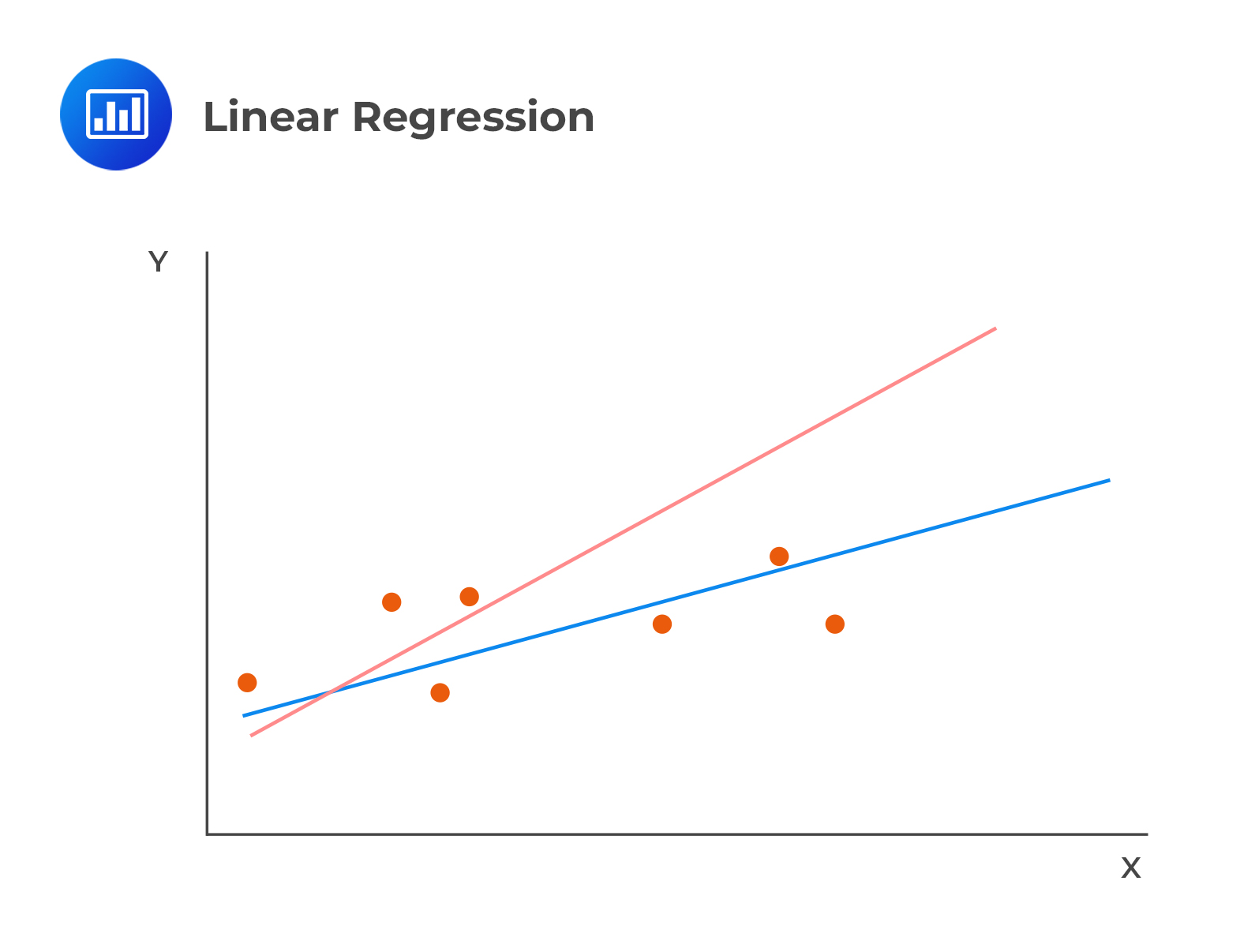
Linear regression calculates a line that best fits the observations. In the following image, the line that best fits the regression is clearly the blue line:

The model chooses the estimated or fitted parameters (\(\beta_0\) and \(\beta_1\)) that minimize the sum of the squared vertical differences between the observations and the regression line (Sum of squared errors (SSE), otherwise referred to as the residual sum of squares). Choosing \(\beta_0\) and \(\beta_1\) occasions the minimization of SSR.
$$
S S E=\sum_{i=1}^{n}\left(Y_{i}-\hat{\beta}_{0}-\hat{\beta}_{1} X_{i}\right)^{2}=\sum_{i=1}^{n}\left(Y_{i}-\hat{Y}_{i}\right)^{2}=\sum_{i=1}^{n} e_{i}^{2}
$$
It is important to remember that \(\beta_0\) and \(\beta_1\) are never observed in a regression model. It is only the estimates, \(\hat{\beta}_0\) and \(\hat{\beta}_1\) that can be observed.
The slope coefficient is defined as the change in the dependent variable caused by a one-unit change in the value of the independent variable. For a regression with one independent variable, the slope coefficient is estimated as shown below.
$$
\hat{\beta}_{1}=\frac{\operatorname{Cov}(X, Y)}{\operatorname{Var}(X)}=\frac{\frac{\sum_{i=1}^{n}\left(Y_{i}-\bar{Y}\right)\left(X_{i}-\bar{X}\right)}{n-1}}{\frac{\sum_{i=1}^{n}\left(X_{i}-\bar{X}\right)^{2}}{n-1}}=\frac{\sum_{i=1}^{n}\left(Y_{i}-\bar{Y}\right)\left(X_{i}-\bar{X}\right)}{\sum_{i=1}^{n}\left(X_{i}-\bar{X}\right)^{2}}
$$
The intercept is the estimated value of the dependent variable when the independent variable is zero. The fitted regression line passes through the point equivalent to the means of the dependent and the independent variables in a linear regression model.
The intercept can, as such, be expressed as:
$$\hat{\beta}_0=\hat{Y}-\hat{\beta}_1\hat{X}$$
Where:
\(\hat{Y}\) = mean of Y.
\(\hat{X}\) = mean of X.
Arth Shah is using regression analysis to forecast inflation based on unemployment data from 2011 to 2020. Shah has computed the following values.
We can calculate and interpret the slope coefficient and the intercept term for the regression analysis as follows:
$$\begin{align} \text{Slope Coefficient}(\hat{\beta}_1) &=\frac{Cov(X, Y)}{(Var (X)}\\ &=\frac{-0.000130734}{0.000144608}=-0.90405\end{align}$$
$$\begin{align} \hat{\beta}_0 &=\hat{Y}-\hat{\beta}_1\hat{X}\\&=0.0234-(-0.90405)\times 0.0526 =0.070953\end{align}$$
Given the value of the slope coefficient, (-0.90405\(\sim\) -0.9), we can say that inflation rates decrease (increase) by 0.90 units whenever unemployment rates increase (decrease) by one unit. littlescholarsnyc.com
Question
A regression model with one independent variable requires several assumptions for valid conclusions. Which of the following statements most likely violates those assumptions?
- The independent variable is random.
- The error term is distributed normally.
- There exists a linear relationship between the dependent variable and the independent variable.
Solution
The correct answer is A.
Linear regression assumes that the independent variable, X, is NOT random. This ensures that the model produces the correct estimates of the regression coefficients.
B is incorrect. The assumption that the error term is distributed normally allows us to easily test a particular hypothesis about a linear regression model.
C is incorrect. Essentially, the assumption that the dependent and independent variables have a linear relationship is the key to a valid linear regression. If the parameters of the dependent and independent variables are not linear, then the estimation of that relation can yield invalid results.
Get Ahead on Your Study Prep This Cyber Monday! Save 35% on all CFA® and FRM® Unlimited Packages. Use code CYBERMONDAY at checkout. Offer ends Dec 1st.