Measures of Central Tendency

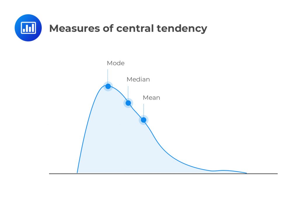
Measures of central tendency are values that tend to occur at the center of a well-ordered data set. As such, some analysts call them measures of central location. Mean, median, and mode are all measures of central tendency. Even then, there are situations where one of them is the most appropriate compared to the others. Among the three measures, the mean is the most common and can also be subdivided into smaller sub-types as we shall see shortly.

Arithmetic Mean

The population mean is the summation of all the observed values in the population, ∑X_i, divided by the total number of observations, N. The population mean differs from the sample mean, which is based on a few observed values ‘n’ that are chosen from the population. Therefore:

$$ \text{Population mean} =\cfrac { \sum { { X }_{ i } } }{ N } $$

$$ \text{Sample mean} =\cfrac { \sum { { X }_{ i } } }{ n } $$

Analysts use the sample mean to estimate the actual population mean.

The population mean and the sample mean are both arithmetic means. The arithmetic mean for any data set is unique and is computed using all the data values. Among all the measures of central tendency, it is the only measure for which the sum of the deviations from the mean is zero.

Example 1: Calculating the Mean

The following are the annual returns on a given asset realized between 2005 and 2015.

12%   13%   11.5%   14%   9.8%   17%   16.1%   13%   11%   14%

1. Calculate the population mean.

2. Compute the sample mean assuming the returns for the first 7 years are unknown, i.e., we only have 13%, 11%, and 14%.

Solution

$$ \begin{align*} \text{Population mean} & =\cfrac {(0.12 + 0.13 + 0.115 + 0.14 + 0.098 + 0.17 + 0.161 + 0.13 + 0.11 + 0.14)}{10} \\ & = 0.1314 \text{ or } 13.14\% \\ \text {Sample mean} & = \cfrac {(0.13 + 0.11 + 0.14)}{3} \\ & = 0.1267 \text{ or } 12.67\% \\ \end{align*} $$

A commonly cited demerit of the arithmetic mean is that it is not resistant to the effects of extreme observations or what we call ‘outsider values.’ For instance, consider the following data set:

{1   3   4   5   34}

The arithmetic mean is 9.4, which is greater than most of the values. This is due to the last extreme observation, i.e., 34.

Weighted Mean

The weighted mean takes the weight of every observation into account. It recognizes that different observations may have disproportionate effects on the arithmetic mean. Therefore:

$$ \text{Weighted mean} = \sum { { X }_{ i }{ W }_{ i } } $$

Example 2: Calculating the Weighted Mean

A portfolio consists of 30% ordinary shares, 25% T-bills and 45% preference shares with returns of 7%, 4%, and 6% respectively. Compute the portfolio return.

Solution

The return of any portfolio is always the weighted average of the returns of individual assets. Therefore:

$$ \text{Portfolio return} = (0.07 * 0.3) + (0.04 * 0.25) + (0.06 * 0.45) = 5.8\% $$

Median

The median is the statistical value located at the center of a set of data that has been organized in the order of magnitude. For an odd number of observations, the median is simply the middle value. If the number of observations is even, the median is the middle point (average) of the two middle values. Unlike the arithmetic mean, the median is resistant to the effects of extreme observations.

Example 3: Calculating the Median

Find the median return in Example 1 above.

Solution

First, we arrange the returns in ascending order:

9.8%   11%   11.5%   12%   13%   13%   14%   14%   16.1%   17%

Since the number of observations is even, the median return will be the middle point of the two middle values:

\( \cfrac {(13\% + 13\%)}{2} = 13\%\)

Mode

Mode is simply the value that occurs most frequently in a set of data. On a histogram, it is the highest bar. A set of data may have a mode or none at all, e.g., the returns in Example 1 above. One of its major merits is that it can be determined from incomplete data, provided we know the observations with the highest frequency.

Example 4: Calculating the Mode

Determine the mode from the following data set:

{20%   23%   20%   16%   21%   20%   16%   23%   25%   27%   20%}

Solution

The mode is simply 20%. It occurs 4 times, a frequency higher than that of any other value in the data set.

Geometric Mean

The geometric mean is a measure of central tendency, mainly used to measure growth rates. We define it as the n^th root of the product of n observations:

$$ \text{GM} ={ \left( { X }_{ 1 }\ast { X }_{ 2 }\ast { X }_{ 3 }\ast { X }_{ 4 }\ast …\ast { X }_{ n-1 }\ast { X }_{ n } \right) }^{ \frac { 1 }{ n } } $$

The formula above only works when we have non-negative values. To solve this problem, especially when dealing with percentage returns, we add 1 to every value and then subtract 1 from the final result.

Example 5: Calculating the Geometric Mean

An ordinary share from a certain company registered the following rates of return over a 6-year period:

-4%   2%   8%   12%   14%   15%

Compute the compound annual rate of return for the period.

Solution

$$ \text{GM} = (0.96 * 1.02* 1.08 * 1.12 * 1.14 * 1.15)^{\frac{1}{6}} = 1.0761 – 1 = 0.0761 \text{ or } 7.61 % $$

Important exam tip: the geometric mean is always less than the arithmetic mean and the gap between the two widens as the variability of values increases.

Harmonic Mean

Analysts use the harmonic mean to determine the average growth rates of economies or assets. If we have N observations:

$$ \text{HM} = \cfrac {N}{ \left(\sum { \frac { 1 }{ { X }_{ i } } } \right)} $$

Example 6: Calculating the Harmonic Mean

For the last three months of 2015, the price of a stock was $4, $5 and $7 respectively. Compute the average cost per share.

$$ \text{HM} =\cfrac {3}{ \left(\frac {1}{4} + \frac {1}{5} + \frac {1}{7} \right)} = $5.06 $$

Important point: harmonic mean < Geometric mean < Arithmetic mean