Hypothesis Testing

A hypothesis is an assumed statement about a population’s characteristics, often considered an opinion or claim about an issue. To determine if a hypothesis is accurate, statistical tests are used. Hypothesis testing uses sample data to evaluate if a sample statistic reflects a population with the hypothesized value of the population parameter.

Below is an example of a hypothesis:

“The mean return of small-cap stock is higher than that of large-cap stock.”

Hypothesis testing involves collecting and examining a representative sample to verify the accuracy of a hypothesis. Hypothesis tests help analysts to answer questions such as:

• Is bond type A more profitable than type B?
• Does staff training lead to improved efficiency at the workplace?
• Are motor vehicle insurance claims consistent with a lognormal distribution?

Procedure Followed During Hypothesis Testing

Whenever a statistical test is being performed, the following procedure is generally considered ideal:

1. Statement of both the null and the alternative hypotheses.
2. Selection of the appropriate test statistic, i.e., what’s being tested, e.g., the population mean, the difference between sample means, or variance.
3. Specification of the level of significance.
4. A clear statement of the decision rule to guide the choice of whether to reject or approve the null hypothesis.
5. Calculation of the sample statistic.
6. Arrival at a decision based on the sample results.

Step 1: Stating the Hypotheses

The Null vs. Alternative Hypothesis

The null hypothesis, denoted as \(H_0\), signifies the existing knowledge regarding the population parameter under examination, essentially representing the “status quo.” For example, when the U.S. Food and Drug Administration inspects a cooking oil manufacturing plant to confirm that the cholesterol content in 1 kg oil packages doesn’t exceed 0.15%, they might create a hypothesis like:

\(H_0\): Each 1 kg package has 0.15% cholesterol.

A test would then be carried out to confirm or reject the null hypothesis.

Typical statements of \(H_0\) include:

$$ \begin{align*}
H_0:\mu& = \mu_0 \\
H_0: \mu & \le\mu_0 \\
H_0: \mu & \geq \mu_0
\end{align*} $$

Where:

\(\mu\) = True population mean.

\(\mu_0\) = Hypothesized population mean.

The alternative hypothesis, denoted as \(H_a\), is a contradiction of the null hypothesis. Therefore, rejecting the \(H_0\) makes \(H_a\) valid. We accept the alternative hypothesis when the “status quo” is discredited and found to be false.

Using our FDA example above, the alternative hypothesis would be:

\(H_a\): Each 1 kg package does not have 0.15% cholesterol.

One-tailed vs. Two-tailed Hypothesis Testing

One-tailed Test

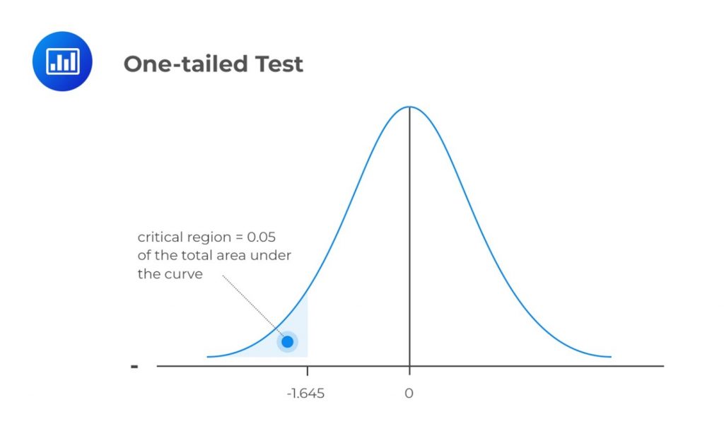
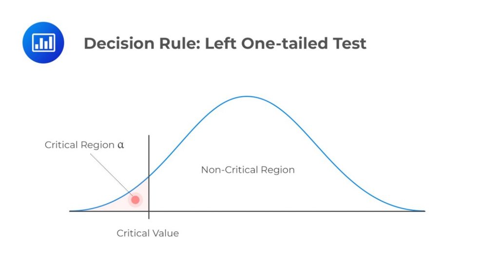
A one-tailed test (one-sided test) is a statistical test that considers a change in only one direction. In such a test, the alternative hypothesis either has a \(\lt\) (less than sign) or \(\gt\) (greater than sign), i.e., we consider either an increase or reduction, but not both.

A one-tailed test directs all the significance levels \((\alpha)\) to test statistical significance in one direction. In other words, we aim to test the possibility of a change in one direction and completely disregard the possibility of a change in the other direction.

If we have a 5% significance level, we shall allot 0.05 of the total area in one tail of the distribution of our test statistic.

Examples: Hypothesis Testing

Let us assume that we are using the standardized normal distribution to test the hypothesis that the population mean is equal to a given value \(X\). Further, let us assume that we are using data from a sample drawn from the population of interest. Our null hypothesis can be expressed as:

$$ H_0: \mu= X $$

If our test is one-tailed, the alternative hypothesis will test if the mean is either significantly greater than \(X\) or significantly less than \(X\), but NOT both.

Case 1: At the 95% Confidence Level

$$ H_a: \mu \lt X $$

The mean is significantly less than \(X\) if the test statistic is in the bottom 5% of the probability distribution. This bottom area is known as the critical region (rejection region). We will reject the null hypothesis if the test statistic is less than -1.645.

Case 2: Still at the 95% Confidence Level

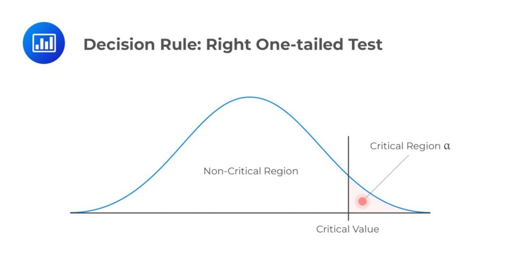
$$ H_{a1}: \mu \gt X $$

We would reject the null hypothesis only if the test statistic is greater than the upper 5% point of the distribution. In other words, we would reject \(H_0\) if the test statistic is greater than 1.645.

A Two-tailed Test

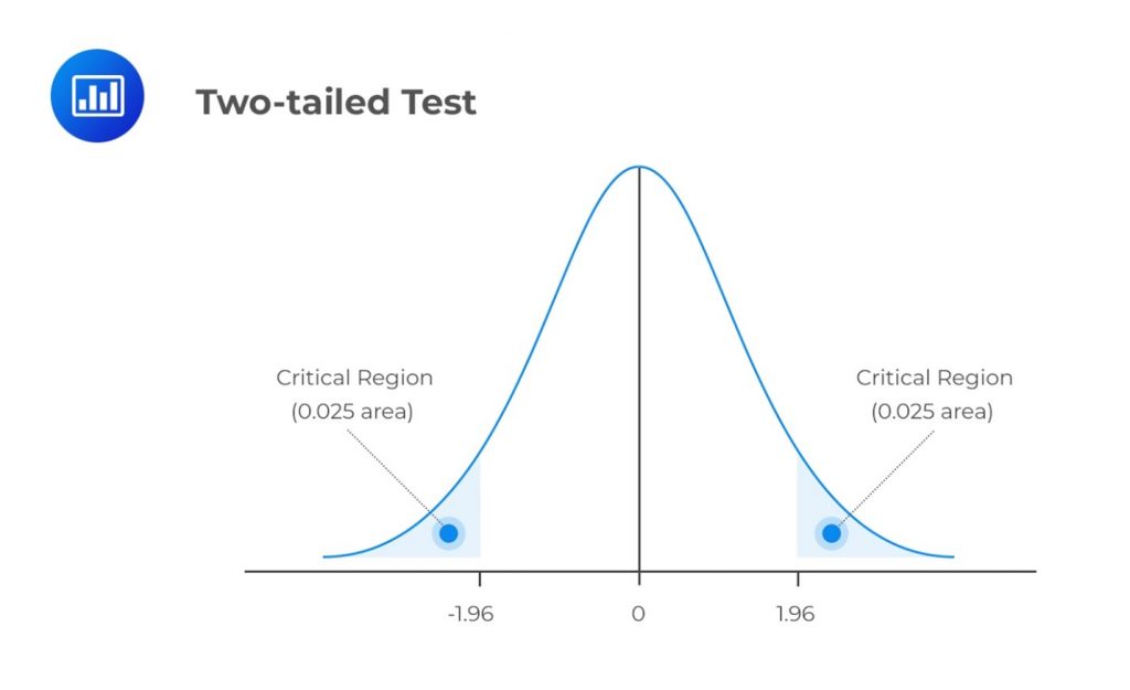
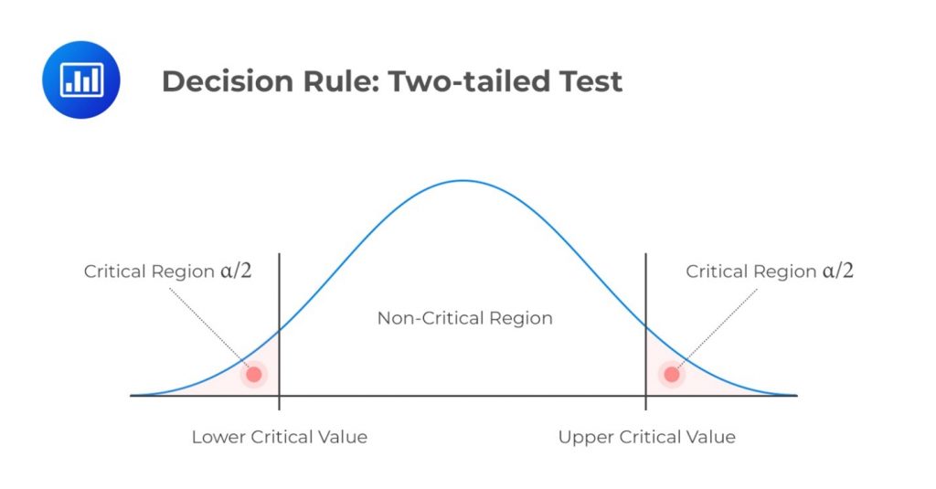
A two-tailed test considers the possibility of a change in either direction. It looks for a statistical relationship in both a distribution’s positive and negative directions. Therefore, it allows half the value of \(\alpha\) to test statistical significance in one direction and the other half to test the same in the opposite direction. A two-tailed test may have the following set of hypotheses:

$$ \begin{align*}
H_0: \mu &= X \\
H_1: \mu & \neq X \end{align*} $$

Refer to our earlier example. If we were to carry out a two-tailed test, we would reject \(H_0\) if the test statistic turned out to be less than the lower 2.5% point or greater than the upper 2.5% point of the normal distribution.

Step 2: Identify the Appropriate Test Statistic and Distribution

Test Statistic

A test statistic is a standardized value computed from sample information when testing hypotheses. It compares the given data with what an analyst would expect under a null hypothesis. As such, the null hypothesis is a major determinant of the decision to accept or reject \(H_0\), the null hypothesis.

We use test statistic to gauge the degree of agreement between sample data and the null hypothesis. Analysts use the following formula when calculating the test statistic for most tests:

$$ \text{Test statistic} =\frac { \text{Sample statistic} – \text{Hypothesized value}}{\text{Standard error}} $$

The test statistic is a random variable that varies with each sample. The table below provides an overview of commonly used test statistics, depending on the presumed data distribution:

$$ \begin{array}{c|c}
\textbf{Hypothesis Test} & \textbf{Test Statistic} \\ \hline
\text{Z-test} & \text{Z- statistic (Normal distribution)} \\ \hline
\text{Chi-Square Test} & \text{Chi-square statistic} \\ \hline
\text{t-test} & \text{t-statistics} \\ \hline
\text{ANOVA} & \text{F-statistic}
\end{array} $$

We can subdivide the set of values that the test statistic can take into two regions: The non-rejection region, which is consistent with the \(H_0\), and the rejection region (critical region), which is inconsistent with the \(H_0\). If the test statistic has a value found within the critical region, we reject the \(H_0\).

As is the case with any other statistic, the distribution of the test statistic must be completely specified under the \(H_0\) when the \(H_0\) is true.

The following is the list of test statistics and their distributions:

$$ \begin{array}{c|c|c|c}
\textbf{Test} & \textbf{Test Statistic} & \textbf{Test Statistic} & \textbf{Number of} \\
\textbf{Subject} & \textbf{Formula} & \textbf{Distribution} & \textbf{Degrees of} \\
& & & \textbf{Freedom} \\ \hline
\text{Single Mean} & t=\frac{\bar{X}-\mu_0}{\frac{s}{\sqrt n}} & t-\text{distribution} & n-1 \\ \hline
\text{Difference in} & t=\frac {(\bar {X_1}-\bar {X_2})-(\mu_1-\mu_2)}{\sqrt{\frac {s_p^2}{n_1}+\frac {s_p^2}{n_2}}} & t-\text{distribution} & n_1+n_2-1 \\
\text{Means} & & & \\ \hline
\text{Mean of} & t=\frac{\bar{d}-\mu_{d0}}{s_{\bar{d}}} & t-\text{distribution} & n-1 \\
\text{Differences} & & & \\ \hline
\text{Single} & \chi^2 =\frac{s^2\left(n-1\right)}{\sigma_0^2} & \text{Chi-square} & n-1 \\
\text{Variance} & & \text{Distribution} & \\ \hline
\text{Difference in} & F=\frac{S_1^2}{S_2^2} & \text{F-distribution} & n_1-1, n_2-1 \\
\text{variances} & & & \\ \hline
\text{Correlation} & t=\frac{r\sqrt{n-2}}{\sqrt{1-r^2}} & \text{t-distribution} & n-2 \\ \hline
\text{Independence} & \chi^2=\sum_{i=1}^{m}\frac{\left(O_{ij}-E_{ij}\right)^2}{E_{ij}} & \text{Chi-square} & \left(r-1\right)\left(c-1\right) \\
\text{(categorical data)} & & \text{Distribution} & \\
\end{array} $$

Where:

\(\mu_0\), \(\mu_{d_0}\), and \(\sigma_{0}^2\) denote hypothesized values of the mean, mean difference, and variance in that order.

\(\bar{X}\), \(\bar{b}\) \(s^2\), \(s\) and \(r\) denote the sample mean of the differences, sample variance, sample standard deviation, and correlation, in that order.

\(O_{ij}\) and \(E_{ij}\) are observed and expected frequencies, respectively, with \({r}\) indicating the number of rows and \(c\) indicating the number of columns in the contingency table.

Step 3: Specify the Level of Significance

The significance level represents the amount of sample proof needed to reject the null hypothesis. First, let us look at type I and type II errors.

Type I and Type II Errors

When using sample statistics to draw conclusions about an entire population, the sample might not accurately represent the population. This can result in statistical tests giving incorrect results, leading to either erroneous rejection or acceptance of the null hypothesis. This introduces the two errors discussed below.

Type I Error

Type I error occurs when we reject a true null hypothesis. For example, a type I error would manifest in the rejection of \(H_0 = 0\) when it is zero.

Type II Error

Type II error occurs when we fail to reject a false null hypothesis. In such a scenario, the evidence the test provides is insufficient and, as such, cannot justify the rejection of the null hypothesis when it is false.

Consider the following table:

$$ \begin{array}{c|c|c}
\textbf{Decision} & {\text{True Null Hypothesis}} & {\text{False Null Hypothesis }} \\
& {(H_0)} & {(H_0)} \\ \hline
\text{Fail to reject the} & \textbf{Correct decision} & \textbf{Type II error} \\
\text{null hypothesis} & & \\ \hline
\text{Reject null} & \textbf{Type I error} & \textbf{Correct decision} \\
\text{hypothesis} & & \\
\end{array} $$

The level of significance, denoted by \(\alpha\), represents the probability of making a type I error, i.e., rejecting the null hypothesis when it is true. The confidence level complements the significance level, \(\left(1-\alpha\right)\).

We use \(\alpha\) to determine critical values that subdivide a distribution into the rejection and the non-rejection regions. The figure below gives an example of the critical regions under a two-tailed normal distribution and 5% significance level:

Consequently, \(\beta\), the direct opposite of \(\alpha\), is the probability of making a type II error within the bounds of statistical testing. The ideal but practically impossible statistical test would be one that simultaneously minimizes \(\alpha\) and \(\beta\).

The Power of a Test

The power of a test is the direct opposite of the significance level. The level of significance gives us the probability of rejecting the null hypothesis when it is, in fact, true. On the other hand, the power of a test gives us the probability of correctly discrediting and rejecting the null hypothesis when it is false. In other words, it gives the likelihood of rejecting \(H_0\) when, indeed, it is false. Expressed mathematically,

$$ \text{Power of a test} = 1- \beta = 1-P\left(\text{type II error}\right) $$

In a scenario with multiple test results for the same purpose, the test with the highest power is considered the best.

Steps 4, 5, 6: State the Decision Rule, Calculate the Test Statistic, and Make a Decision

The decision rule is the procedure that analysts and researchers follow when deciding whether to reject or not reject a null hypothesis. We use the phrase “not to reject” because it’s statistically incorrect to “accept” a null hypothesis. Instead, we can only gather enough evidence to support it.

Breaking Down the Decision Rule

The decision to reject or not reject a null hypothesis relies on the distribution of the test statistic. The decision rule compares the calculated test statistic to the critical value.

If we reject the null hypothesis, the test is considered statistically significant. If not, we fail to reject the null hypothesis, indicating insufficient evidence for rejection.

We use the test’s significance level if a variable follows a normal distribution. This helps us find critical values corresponding to specific points on the standard normal distribution. These critical values guide the decision-making process for rejecting or not rejecting a null hypothesis.

Before deciding whether to reject or not reject a null hypothesis, it’s crucial to determine whether the test should be one-tailed or two-tailed. This choice depends on the nature of the research question and the direction of the expected effect. Notably, the number of tails determines the value of \(\alpha\) (significance level). The following is a summary of the decision rules under different scenarios.

Left One-tailed Test

\(H_a: \text{ Parameter } \lt X\)

Decision rule: Reject \(H_0\) if the test statistic is less than the critical value. Otherwise, do not reject \(H_0\).

Right One-tailed Test

\(H_a: \text{ Parameter } \gt X\)

Decision rule: Reject \(H_0\) if the test statistic is greater than the critical value. Otherwise, do not reject \(H_0\).

Two-tailed Test

\(H_a: \text{ Parameter } \neq X \text{ (not equal to X) }\)

Decision rule: Reject \(H_0\) if the test statistic is greater than the upper critical value or less than the lower critical value.

The p-Value in Hypothesis Testing

The p-value is the lowest level of significance at which we can reject a null hypothesis. The probability of coming up with a test statistic would justify our rejection of a null hypothesis, assuming that the null hypothesis is indeed true.

Breaking Down the p-value

When carrying out a statistical test with a fixed value of the significance level (α), we merely compare the observed test statistic with some critical value. For example, we might “reject an \(H_0\) using a 5% test” or “reject an \(H_0\) at a 1% significance level.” The problem with this ‘classical’ approach is that it does not give us details about the strength of the evidence against the null hypothesis.

Determination of the p-value gives statisticians a more informative approach to hypothesis testing. The p-value is the lowest level at which we can reject an \(H_0\). This means that the strength of the evidence against an \(H_0\) increases as the p-value becomes smaller.

In one-tailed tests, the p-value is the probability below the calculated test statistic for left-tailed tests or above the test statistic for right-tailed tests. For two-tailed tests, we find the probability below the negative test statistic and add it to the probability above the positive test statistic. This combines both tails for the p-value calculation.

Example: p-value

\(\theta\) represents the probability of obtaining a head when a coin is tossed. Assume we tossed a coin 200 times, and the head came up in 85 out of the 200 trials. Test the following hypothesis at a 5% level of significance.

\(H_0:\ \theta = 0.5\)

\(H_1:\ \theta \lt 0.5\)

Solution

First, note that repeatedly tossing a coin follows a binomial distribution.

Our p-value will be given by \(P(X \lt 85)\), where \(X\) follows a binomial (200,0.5), assuming the \(H_0\) is true.

$$ \begin{align*}
&= P \Bigl \lceil Z \lt \frac {(85.5 – 100)}{\sqrt{50}} \Bigl \rceil \\
&= P\left(Z \lt -2.05\right)= 1 – 0.97982 = 0.02018
\end{align*} $$

(We have applied the Central Limit Theorem by taking the binomial distribution as approximately normal.)

Since the probability is less than 0.05, the H0 is extremely unlikely, and we have strong evidence against an \(H_0\) that favors \(H_1\). Therefore, clearly expressing this result, we could say:

“There is very strong evidence against the hypothesis that the coin is fair. We, therefore, conclude that the coin is biased against heads.”

Remember, failure to reject a \(H_0\) does not mean it is true. It means there is insufficient evidence to justify the rejection of the \(H_0\) given a certain level of significance.

Question

A CFA candidate conducts a statistical test about the mean value of a random variable \(X\).

\(H_0: \mu = \mu_0 \text{ vs } H_1: \mu \neq \mu_0\)

She obtains a test statistic of 2.2. Given a 5% significance level, determine the p-value.

1. 1.39%.
2. 2.78.
3. 2.78%.

Solution

The correct answer is C.

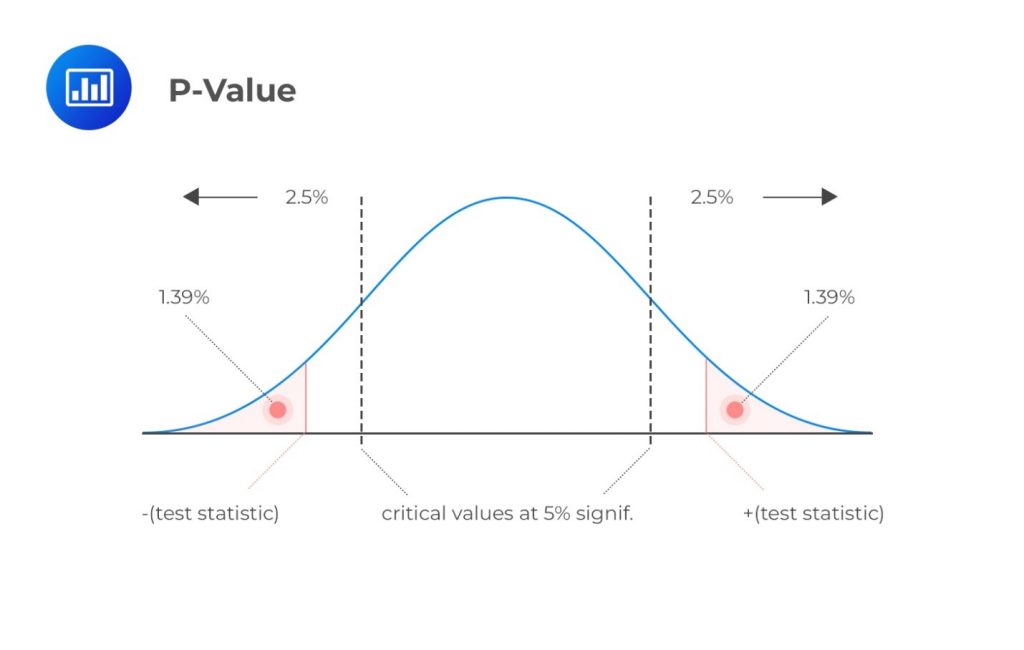
$$ \text P-\text{value}= P(Z \gt 2.2) = 1 – P(Z \lt 2.2) = 1.39\% \times 2 = 2.78\% $$

(We have multiplied by two since this is a two-tailed test.)

Interpretation: The p-value (2.78%) is less than the significance level (5%). Therefore, we have sufficient evidence to reject the \(H_0\). In fact, the evidence is so strong that we would also reject the \(H_0\) at significance levels of 4% and 3%. However, at significance levels of 2% or 1%, we would not reject the H0 since the p-value surpasses these values.